|
Structural Bioinformatics Library
Template C++ / Python API for developping structural bioinformatics applications.
|
|
Structural Bioinformatics Library
Template C++ / Python API for developping structural bioinformatics applications.
|
In the following, we provide the main concepts and the terminology used in the SBL.
These concepts are a good starting point for anyone whishing to make use of the SBL
Let's introduce the general terminology used throughout the library.
Molecular systems.
Our journey starts with collections of atoms/particles, handled using the package Molecular_system, which provides a hierarchical organization.
Molecular labels.
Several tasks require defining groups of atoms, e.g. identifying rigid regions within a molecule, studying the interface between two partners, etc. We define groups such groups of atoms using molecular labels, see Molecular Labeling and MolecularSystemLabelsTraits.
Covalent structures.
Molecules are made of bonds connecting atoms, which yields a natural encoding in terms of graphs, as done in the package Molecular_covalent_structure (class SBL::CSB::T_Molecular_covalent_structure).
In general, the graph is associated with one or several molecules; in this latter case, it contains as many connected components as individual molecules.
This topological representation makes it possible to iterate on the individual molecules, and within a molecule, iterate on particles, bonds, bond angles and torsion angles.
Conformations and geometric information.
The geometry of a molecule corresponds to the embedding of the molecular graph in 3D, which is specified with the Cartesian coordinates of the atoms. This embedding is called molecular conformation Molecular_conformation (class SBL::Models::T_Geometric_conformation_traits::Conformation) for short.
Practically, this geometric information is used in two main classes of applications:
Collections of atoms: this first group of applications, see Space Filling Model, merely require the positions and radii of these atoms. Such models are called space filling models, see Work Package: Space Filling Models.
Annotations from biochemistry and chemistry.
Applications in bioinformatics often require biological and/or biochemical annotations. The following packages are of interest:
Annotations from biochemistry and chemistry.
The coherence between the aforementioned pieces of information ( molecular system, covalent structure, conformation) is handled by higher level classes, including SBL::CSB::Polypeptide_chain_representation and SBL::CSB::Protein_representation from the package Protein_representation.
A molecular labeling is a grouping of the particles of a molecular structure. Such grouping are used when the groups formed have specific properties, or when one wishes to investigate interactions between such groups.
Given a molecular structure, a set of labels 

The labels may have a hierarchical structure, in which case they are represented as (a forest of) trees. In that case, we distinguish between primitive labels and hierarchical labels. The set of all primitive labels is denoted 


Given a list of particles 


In this respect, the molecular system associated with a label 


Practically, a number of classifiers defining molecular systems are provided. These classifiers follow a generic pattern (a C++ concept to perform a hierarchical decomposition), as defined in the package MolecularSystemLabelsTraits.
In the SBL, each particle is annotated with properties. Depending on the context, the annotations may be compulsory or optional.
A compulsory annotation is such that memory space to store it within each particle is allocated at compile time to store it. As the name suggests, such annotations are mandatory in a given context. See section Compulsory Annotations for more details about compulsory annotations.
As an example, one may consider the case of particles represented by 3D balls: annotating such particles with a radius is mandatory. See section Atomic Radii and Group Radii for more details.
On the opposite, optional annotations are loaded on the fly – no storage reserved at compile time. Such annotations are typically used to further analyze the results of a SBL program. Optional annotations are dynamics, i.e. dynamically loaded using the option –annotations-file, while running the SBL program. Note that any number of annotations can be loaded just by repeating the option for each annotation file.
As an example of optional annotations, one may consider solvation parameters, on a per particle (atom) basis. See section Optional Annotations for more details.
A precise description of the annotation's system is described in the package ParticleAnnotator.
A space filling model is a molecular geometric model where each particle is represented by a 3D ball. Such models are of special interest to represent molecular surfaces and volumes, as well as interfaces. In the SBL, applications using space filling models are grouped in the Applications page Space Filling Model .
In the sequel, we review some basic facts about these models. For a discussion of such models from the biophysical standpoint, the reader may consult [101] as well as [100] and the references therein. For a treatment of selected aspects of such models, 
A finite family of balls is denoted 


The boundary operator is denoted 


We note that in the SBL, space filling models are key in the following two packages:
In a space filling model, the radius of a particle typically depends on the atomic type and on its covalent environment.
In dealing with crystal structures, the radii may be adapted, depending on the presence or not of hydrogen atoms. When all H atoms have not been reported, which is in general the case, a common strategy consists of using so-called group radii: the group radius of one heavy atom accounts for its own size together with that of the H atoms it is covalently bonded to, see [62] .
In the SBL, the radii of particles are annotations attached to the particles, loaded from a file specifying the radius for each particle type. In particular, the class SBL::Models::T_Radius_annotator_for_particles_with_annotated_name allows:
to load the radii from a specification file, or to load default radii if no file is given (default radii are the ones from [62] , see SBL::Models::T_Radius_annotator_for_particles_with_annotated_name),
to add a constant value to all loaded radii (e.g for accounting for a water probe, by adding 1.4 to all radii, see section Solvent Accessible Model),
For atoms, two group radii are available: from Chothia et al in 1975 [63] (the default ones, available here), and from Tsai et al in 1999 [188] (avalaible here). When using pseudo-atoms representing the residues, there is one radius per residue type. The radius of an amino acid is computed as the radius of a 3D sphere from the average volume of the residue [167] (available here).
The Solvent Accessible Model (SAM) is a molecular geometric model where the particle radii are expanded by the mean radius of a water molecule (circa 
The Solvent Accessible Surface (SAS) of a SAM is the boundary of the balls defining the SAM. The SAS consists of spherical polygons, circle arcs (found at the intersection of two spheres), and vertices (found at the intersection of three spheres), as defined in the package Union_of_balls_boundary_3. The area of the SAS is called the Solvent Accessible Surface Area (SASA) .
Consider two partners 


See also the Buried_surface_area package for more details.
Using this model, the core and the rim of an interface are easily defined [136] : the rim consists of the particles retaining solvent accessibility in the complex, while the core consists of the particles which are buried in the complex.
This model is related to Voronoi models of interfaces [47] , [31] , and [54] , which may be seen as improvements in several respects, in particular:
selected particles which are buried in their own sub-unit can be found at the interface.
In the SBL, topics related to conformational analysis are studied in the more general setting of energy landscapes [194].
The SBL provides numerous tools to sample EL and study the resulting sets of conformations, as detailed in [50] and [170].
The corresponding applications are gathered in the part Conformational Analysis. The corresponding C++ code hinges on the following concepts:
Conformations and their representations
Energy landscapes and their representations
Algorithms to explore energy landscapes
Conformations and their representation in Cartesian or internal coordinates. We consider a macromolecular system 


In Cartesian coordinates, each atom is attributed 3 coordinates (x, y ,z). In internal coordinates – also known as Z-matrix, see [158], the atoms of a molecule are rather described using bond distances between two atoms, bond angles between three atoms and torsion angles between four atoms – see Fig. fig-internal-coordinates . It is possible to switch from a coordinates system to another one by applying a transformation. However, each transformation requires an information that is not encoded in the original coordinates system.
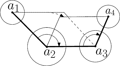 |
| Internal coordinates representation: illustration for a system of four atoms The four atoms are    |
Moving from internal coordinates to cartesian coordinates. This transformation requires the cartesian coordinates of the first three atoms:
The first atom corresponds to the origin of the coordinate system. Practically, its three Cartesian coordinates are set to zero.
The second atom is at a fixed distance from the first one (their bond distance), so that there are two degrees of freedom left. Practically, one may set the x value to distance, and the remaining two coordinates to zero.


Moving from cartesian coordinates to internal coordinates. Assume that the topology of the molecule (the bonds) is known. From this topology, internal coordinates can be computed for each bond (its bond length), for each pair of consecutive bonds (their bond angle), and for each triple of consecutive bonds (their torsion angle).
The class SBL::CSB::T_Molecular_internal_coordinates allows to compute individually each bond length, bond angle and torsion angle.

Comparing conformations. In general the distance between two conformations is denoted 


Sampling. In the context of the SBL, a sampling refers to a set of conformations. It may also be called a conformational ensemble , even though it does not carry any statistical property.
A conformational ensemble , also called sampling 

Whenever a local energy minimizer is available, that is, when the conformations can be quenched, the associated set of quenched conformations is denoted 

If Cartesian coordinates are used, the conformations in 


Once a one-to-one correspondence between the atoms of 
Nearest neighbor graph. We define:
That is, a NNG connects conformations in the configuration space 

Landscape and potential energy landscape (PEL). We define an energy landscape [194], or landscape for short, as a triple:
conformational space
a height function 
distance function 
The height function 


Critical points and their connexions. If the gradient of the height function vanishes at
For a given minimum, or particular interest is the lowest transition state that directly connects it to a minimum of lower energy:
If 

Discrete representations involving samples. Various constructions can be carried out by combining samplings and energies.
A lifted sample is a sample equipped with a real number, called its height. When this number represents the potential energy, a collection of such samples is called a sampled energy landscape.
Also, using the connectivity of a NNG to connect lifted samples results in a lifted NNG. For example, if the height is the potential energy, the lifted NNG defines a network on the PEL.
Discrete representations involving critical (i.e., stationary) points only. Of special interest on a landscape are the local minima and the transition paths connecting them. In the smooth setting, a transition between two local minima corresponds to the existence of an integral curve joining the saddle to the minimum. More specifically, in Morse theory [144], these curves define the so-called unstable manifold of the saddle. Generically, two such curves are found for each saddle – note however that they may end up in the same local minimum, a situation we refer to as a bump transition (Fig. fig-bump-middle-slope-bassin).


Note that in a compressed TG, all vertices correspond to local minima, while every edge corresponds to two minima which are connected through a saddle in the TG. As we shall see, such compressed graphs are useful to derive a number of properties of EL, and also to compare them.
For a number of tasks related to the analysis of energy landscapes, it is useful to think of the TG as a bipartite graph:
This definition calls for two comments:
In computational topology [16], the MSW complex is the mathematical object allowing one to efficiently compute the homology of sublevel sets of a manifold, from a function defined on that manifold – in our case the conformational space and the energy. The MSW complex involves critical points of all indices, but for energy landscapes, we shall mainly use local minima and index one saddles.
Selected saddles associated with a transition graph can also be used to define the following:
The following comments are in order:
The forest associated with a DG has a single tree when the TG is connected.
Generically, in the context of smooth Morse theory, a key saddle is linked to two local minima, which may coincide. Practically, degeneracies where the key saddles is linked to more local minima may be encountered.
Several important operations can be carried on landscapes, including:
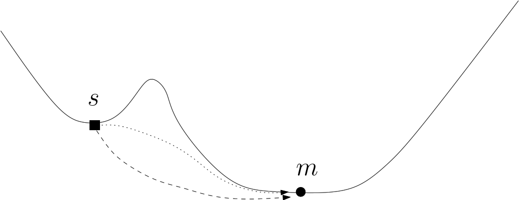 |
| A loop around a saddle Note that the dotted path is located behind the bump of this fictitious 2D landscape. |
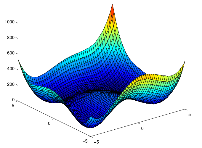 |
| The Himmelblau function: landscape The function is defined by:  |
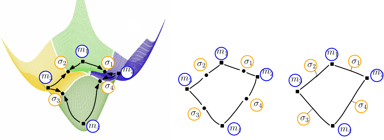 |
| Himmelblau: (Compressed) Transition graph (A)The landscape of Himmelblau, decomposed into the catchment basins of the four local minima (B)The transition graph, with one node for each critical (i.e., stationary) point (C)The compressed transition graph, where the information associated with saddles is stored in the edges joining local minima. |
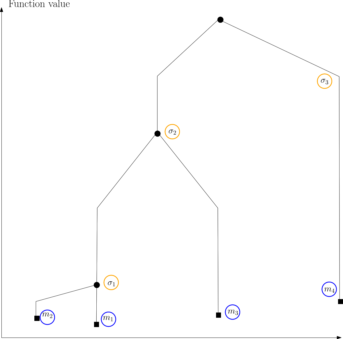 |
| Himmelblau: disconnectivity graph |

Loading structures and geometric models consists of converting structures and geometric models stored in a file into main memory data structures.
As seen from Fig. fig-terminology-loader, loading involves three ingredients, namely:
In the following, we will detail the information contained in the different loadable file formats, and in which contextes they can be used.
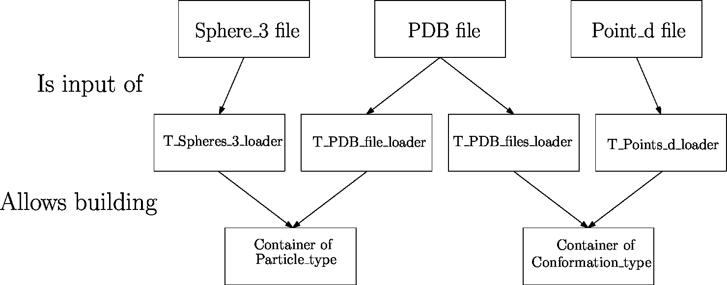 |
| Data flow from files to data structures The files (first row) containing the data are loaded using loaders (second row) into internal data structures. Then, builders transform these internal data structures into data structures (third row) that are usable by the different components of the SBL. Depending on the context, these data structures may be defined by different models (last row). |
The Protein Data Bank is the reference resource for structures of macro-molecules and their complexes. For general information on structures, one may consult : Introduction to Biological Assemblies and the PDB Archive
For information on the PDB file format, one may consult:
In the SBL, the PDB files are loaded into C++ data structures using the class SBL::Models::T_PDB_file_loader: this class uses the (ESBTL) for parsing PDB files and uses parsimonious data structures to store the hierarchical information contained in a PDB file. See the documentation of the class SBL::Models::T_PDB_file_loader for a more detailed description of the available options.
A molecule loaded using the class SBL::Models::T_PDB_file_loader is represented by the ESBTL class ESBTL::Molecular_model . Two comments are in order.
Multiple models. First, if a molecule is represented by several models in the PDB file, one instance of ESBTL::Molecular_model is created for each model. It is possible to access to these data structures using the method SBL::Models::T_PDB_file_loader::get_geometric_model .
Conversions. Depending on the context, the PDB format may have to be converted to a different data format, using a builder. Such a class takes as input an instance of ESBTL::Molecular_model, and fills an output data structure dedicated to a particular context.
For example, in Work Package: Space Filling Models, the data structure can be a container of particles, each particle being represented by a 3D ball – see SBL::Models::T_Atom_with_flat_info_traits::Atom_with_flat_infos_builder . In Work Package: Conformational Analysis, the data structure can be a conformation, that is represented by a D-dimensional point – see SBL::Models::T_Conformation_as_d_point_traits::Conformation_as_d_point_builder .
In the SBL, the applications implement combinatorial, geometric and topological in a biophysical context. While loading a PDB file gives a great number of biophysical properties, one may use the applications on molecules stored in much more basic formats. The simplest format for representing a particle is a 3D ball (or its bounding 3D sphere). A file listing 3D spheres as follows:
x_1 y_1 z_1 r_1
...
can be loaded using the loader SBL::Models::T_Spheres_3_file_loader .
The class SBL::Models::T_Geometric_particle_traits defines a particle reduced to its geometric representation. Then, it is possible to annotate these geometric particles using the annotators provided by the package ParticleAnnotator, as explained in section Decorating Models .
When dealing with conformations, the same problem as section Loading 3D spheres occurs. The simplest format for representing a conformation is a D-dimensional point, also known as the Point_d format, which concatenation all coordinates of the particles of a line. As an example, in dimension say 6, one line reads as :
6 x_1 y_1 z_1 x_2 y_2 z_2
...
can be loaded using the loader SBL::Models::T_Points_d_file_loader .
The class SBL::Models::T_Geometric_conformation_traits defines a conformation reduced to its geometric representation.
When using the programs of the SBL, one may want to decorate the particles of the input molecule(s) to analyze the output as a function of some properties. For example, to compute the ratio of buried residues in a protein that are hydrophobic, one may use the program 
The SBL offers the possibility to annotate dynamically the particles of a molecule with user-defined properties. The term dynamical refers to the possibility to load new properties when starting the program, and to decorate each particle with this new property. It is opposed to static that refers to properties that are already decorating the particles, but that can be modified (e.g, the atomic group radii). Therefore, an atom that is reported in an output file will be reported with all its annotations.
In all the programs of Space Filling Model, dynamical properties can be loaded using the option –annotations-file <path/to/file>. A file describing such properties has to follow simple rules, as shown in the following example:
# First line: 3 keywords i.e. (i) annotation name (ii) key composition (iii) type of annotation
# Subsequent lines:
hydrophobicity RES_NAME char
ALA H
ARG C
GLU P
...
For more details on annotations, see the package ParticleAnnotator.
The SBL uses intensively the Boost Serialization for saving and loading the data structures of the different programs. In the Boost Serialization,
"the term serialization means the reversible deconstruction of an arbitrary set of C++ data structures to a sequence of bytes."
The file containing this sequence of bytes is called an archive. There are three main file formats for an archive: plain text, binary and XML.
In the SBL, the serialization is used for two different goals:
for saving a data structure in an archive, that will possibly be loaded by another program of the SBL,
Since input files for PALSE are XML files, all the archives in the SBL are XML files. In the following, two issues are discussed:
some data structures cannot be fully saved into an archive, and cannot be loaded again – see section Partial Serialization,
While the serialization is a powerful framework for saving and loading data structures, it is not always possible to do so due to the complexity of some data structures. In the following, we introduce the terminology to handle such cases.
In order to serialize an atom as in the previous example, one has to serialize the residue containing it. The process may be recursive, unwinding the hierarchy residue > chain > model > molecular structure.
A is hierarchical iff A has an attribute of type B such that A borrows B and B owns A.
A data structure is termed partially serializable when it cannot be serialized because it is hierarchical. In other words, when the data structure in memory is saved into a file, the pieces of information saved are not sufficient to reconstruct the data structure in main memory from that file. In our previous example, the atom will not be able to access the information on its residue.
Partially serializable data structures use also the Boost Serialization for saving data : the only difference with serializable data structures is that they cannot be loaded from a file.
Another problem encountered in serializing data is the amount of information contained within an archive.
For example, an archive listing the atoms of a molecule contains all the properties of the atom in order to reconstruct in memory this atom. However, when analyzing the output of a program of the SBL with PALSE, the different analysis may not require all the pieces of information contained in the archive.
As a second example, consider an archive listing thousands of conformations of a molecule involving of the order of one thousand atoms: the corresponding archive contains millions of lines and is hard to navigate through.
A solution provided by the SBL consists in storing the information contained in a data structure in at least two different archives:
the main archive contains reduced information where the heavy part is replaced by a simple index,
Saving in multiple archives. The class SBL::IO::T_Multiple_archives_serialization_xml_oarchive provides functionalities to save a serializable data structure into multiple archives. There are two ways to store a serializable data structure:
by providing the paths to both the main and the secondary archives when constructing an instance of SBL::IO::T_Multiple_archives_serialization_xml_oarchive,
by providing only the path to the main archive, in which case the information that is not in the main archive is lost.
In the last case, the data structure cannot be loaded since the information is lost.
Loading from multiple archives. The class SBL::IO::T_Multiple_archives_serialization_xml_iarchive provides functionalities to load a serializable data structure from multiple archives. The only way to load a serializable data structure is to specify the path to the main and secondary archives when constructing an instance of SBL::IO::T_Multiple_archives_serialization_xml_iarchive .
For more detailed information on multiple archives serialization, see the package Multiple_archives_serialization .