Binding_affinity_prediction

Authors: S. Marillet and P. Boudinot and F. Cazals

Goals: Generating and evaluating predictive models for binding affinity

This package provides tools to (i) select binding affinity prediction models from atomic coordinates, typically crystal structures of the partners and/or of the complex, and to (ii) exploit such models to perform affinity predictions.

At the selection stage, given a set of predefined variables coding structural and biochemical properties of the partners and of the complex, the approach consists of building sparse regression models which are subsequently evaluated and ranked using repeated cross-validation [135] .

At the exploitation stage, the variables selected are used to build a predictive model on a training dataset, and predict the affinity on a test dataset.

More precisely, the approach runs through 3 steps:

Pre-processing: a set of complexes is pre-processed, so as to compute the variables used in the model selection and/or exploitation.
Model selection: sparse regressors using subsets of the previous variables are built, and the best ones selected.
Model exploitation: given a set of variables selected from a given dataset, affinity predictions on another dataset can be performed.

General pre-requisites

Binding affinity and dissociation free energy

Consider two species and forming a complex . The dissociation is defined by $\Kd = [A][B]/[AB]$ , namely the ratio between the concentration of individual partners and bound partners.

The strength of this association is quantified by the dissociation free energy $\deltaGd$ , which, in the $c^{\circ} = 1M$ standard state, satisfies with Boltzmann's constant and the temperature:

This equation shows that $\deltaGd$ has two components respectively coding the enthalpic ( $\Delta H$ ), and entropic ( $\Delta S$ ) changes upon binding. As stated above, we wish to estimate these quantities from atomic coordinates, typically crystal structures of the partners and/or the complex.

Key geometric constructions

Parameters

The parameters used in this package are based on the following key geometric constructions:

Solvent accessible surface and its area. The solvent accessible surface of a molecular model is the boundary of its constituting balls. The associated surface area ( $\text{\SASA}$ for short) is the sum of the surface areas exposed by the individual atoms. Upon complex formation, the buried surface area (BSA) is the surface area of the partners buried at the interface, namely the $\text{\SASA}$ lost by the individual atoms. The solvent accessible surface areas are computed using $\text{\sblvorlumepdb}$ . See section Solvent Accessible Model for more details
Buried surface and binding patches. Upon formation of a complex, the BSA is the surface area of the partners which gets buried. Also, the exposed surface of the atoms contributing to the BSA define a binding patch (patch for short) [30] . The BSA and binding patches are computed using $\text{\sblvorshellE}$ . See section Interfaces, Buried Surface Area, and Core-rim Models for more details.
Atomic packing. Consider the Voronoi (power) diagram of an atomic model, using its solvent accessible representation. The restriction of an atom as the intersection between its ball in the solvent accessible model and its cell in the Voronoi diagram. We denote $\volumeb{a}$ (resp. $\volumeu{a}$ ) the volume of the Voronoi restriction of an atom in the bound form (resp. unbound form). The volumes are computed using $\text{\sblvorlumepdb}$ .
Shelling order (SO). The shelling order of an atom from a binding patch is its least distance, counted in integer steps, to the nearest atom from the non-interacting surface (NIS, atoms which are not located at the interface). That is, the atoms on the border of the patch have a SO of 1 and the remaining ones have a Thus, the SO generalizes core-rim models [110] , since the rim corresponds to , and the core to . The shelling order of interface atoms is computed using $\text{\sblvorshellE}$ . See section Interfaces, Buried Surface Area, and Core-rim Models for more details.

Using the previous notions, we define four categories of atoms of a complex:

For interface atoms, denoted $\interf$ , we define two groups, those found on the rim ( $\calI, SO=1$ ), retaining solvent accessibility, and the remaining ones ( $\calI, SO>1$ ).
For the set of non interface atoms, denoted $\notinterf$ , we distinguish between those retaining solvent accessibility ( $\notinterf$ and $\SASA>0$ in the complex), and those which do not ( $\notinterf$ and $\SASA = 0$ in the complex).

Biophysical rationale.

Before defining our parameters, we raise several simple observations underlying their design:

Generalizing the BSA. The BSA is known to exhibit remarkable correlations with various biophysical quantities of protein complexes [110] . However, it does not account for the interface geometry, as the same surface area may be observed for morphologies as diverse as a perfectly isotropic patch, or a long and skinny patch, letting alone curvature. The obliviousness to interface morphology is intuitively detrimental, since morphology relates to the cooperativity of phenomena inherent to non-bonded interactions. As we shall see below, we define a parameter generalizing the BSA by taking into account the SO of interface atoms and their packing properties.
Packing. A closely packed environment yields favorable interactions by increasing the number of neighbors. But it also entails an entropic penalty for that atom, illustrating the classical enthalpy - entropy compensation, which holds in particular for biological systems involving weak interactions [80] [58] . We therefore use atomic volumes and their variations upon binding (Eq. (eq-atom-volume-variation)) to model both the interaction energy and the entropic changes upon binding.
Entropy. Assessing entropic variations requires taking several components into account, in particular configurational entropy and vibrational entropy. Large conformational changes yielding structured elements correspond to entropic penalties, and can be assessed using the root mean square deviation of interface atoms ( $\irmsd$ ). In the sequel, we refine this measure using atomic packing properties. Indeed, packing properties are intuitively related to the vibrational entropy of atoms.

Associated variables

Using the quantities defined in section General pre-requisites, we define the following variables:

Interface terms.

$\text{\IVWIPL}$ , see Eq. (eq-ivwipl): the sum over interface atoms of their shelling order normalized by their packing. Note that since a packed interface is more likely to result in a high affinity, the shelling order is weighted by the inverse of the volume, yielding the inverse volume-weighted internal path length .
$\text{\irmsd}$ = Interface RMSD : the least RMSD for interface atoms.

Packing terms.

Consider the volume variation of $\diffvol{a}$ , see Eq. (eq-atom-volume-variation). As recalled above, packing properties are important in several respects. Adding up volume variations yields the following four sum of volumes differences (VD) parameters:

$\text{\svdsoo}$ ( $\calI, SO(a)=1$ ; Eq. (eq-svdsoo)): sum of VD for the rim interface atoms.
$\text{\svdsogto}$ ( $\calI, SO(a)>1$ ; Eq. (eq-svdsogto)): sum of VD for interface atoms in the interface core.
$\text{\svdnibur}$ ( $\notinterf, \SASA{a} = 0$ ; Eq. (eq-svdnibur)): sum of VD for buried non interface atoms.
$\text{\svdnisurf}$ ( $\notinterf, \SASA{a}>0$ ; Eq. (eq-svdnisurf)): sum of VD for exposed non interface atoms.

Solvent interactions and electrostatics.

The interaction between a protein molecule and water molecules is complex. In particular, the exposition to the solvent of non-polar groups hinders the ability of water molecules to engage into hydrogen bonding, yielding an entropic loss for such water molecules. We define the following terms:

$\text{\NISPOL}$ , see Eq. (eq-nispol): the fraction of charged a.a. on the non interacting surface, as defined in [118] .
$\text{\NISCHAR}$ , see Eq. (eq-nischar): the fraction of polar a.a. on the non interacting surface [118] .
$\text{\POLARSASA}$ , see (Eq. (eq-polar_sasa): an intermediate-grained description of the non-interacting surface which consists in the atomic-wise polar area of the complex. The corresponding term, $\text{\POLARSASA}$ (Eq. (eq-polar_sasa)), is a weighed sum of exposed areas.
$\text{\NISPOLDIFF}$ , see Eq. (eq-nispoldiff): variation of $\text{\NISPOL}$ , to account for conformational changes upon binding,
$\text{\NISCHARDIFF}$ , see Eq. (eq-nischardiff): variation of $\text{\NISCHAR}$ , to account for conformational changes upon binding,
$\text{\SOLVEISEN}$ , see Eq. (eq-solvation_eisenberg): To challenge amino-acid terms with their atomic counterparts and see which ones are best suited to perform affinity predictions, we also included the atomic solvation energy from Eisenberg et al [90] , describing the free energies of transfer from 1-octanol to water per surface unit ( $\text{\AA}$ ). The corresponding variable, $\text{\SOLVEISEN}$ , is a weighted sum of atomic solvent accessible surface areas (Eq. (eq-solvation_eisenberg)), and may be seen as the atomic-scale counterparts of $\text{\NISCHAR}$ and $\text{\NISPOL}$ .

Parameters used to estimate binding affinities.

There are three groups of parameters (see the next equations for their definition):

atomic level parameters : $\text{\IVWIPL}$ , $\text{\svdsoo}$ , $\text{\svdsogto}$ , $\text{\svdnibur}$ , $\text{\svdnisurf}$ , $\text{\SOLVEISEN}$ and $\text{\POLARSASA}$ .
residue level parameters : $\text{\NISPOL}$ , $\text{\NISCHAR}$ , $\text{\NISPOLDIFF}$ and $\text{\NISCHARDIFF}$ .
interface level parameter : $\text{\irmsd}$ .

The acronyms read as follows (see text for details):

Sum of Volume Differences;
Shelling Order;
Inverse Volume Weighted;
Internal Path Length;
Non Interacting Buried/Exposed;
Non Interacting Surface;
Solvent Accessible Surface Area;

Matchings for atoms

For variables describing a change between the bound and unbound forms of the partners e.g. $\text{\svdsoo}$ or $\text{\NISCHARDIFF}$ , it is necessary to match the atoms of the bound partners to those of the unbound partners. For this, the amino-acid sequences of the partners are extracted from the PDB files and aligned. Then, the atoms of every pair of corresponding residues are matched using their name.

Since missing residues and missing atoms are common in crystal structures, the proportion of matched atoms is computed as to investigate potential wrong matchings, and discard entries for which the alignment is not good enough.

Using the programs to pre-process structural data

In this section we explain how to compute the variables presented in section Associated variables .

This step consists of two sub-steps:

$\text{\bapERun}$ : Variables describing geometrical and physico-chemical are computed, using various constructions provided in the SBL. Two settings are supported:
- Crystal structures of the complex and the unbound partners are given,
- Only the crystal structure of the complex is given.
$\text{\bapECompile}$ : Information from the individual runs is assembled. The result may be seen as a matrix of complexes, each defined by its variables.

In section Input: specifications and file types, we explain how other variables can be used.

Input: specifications and file types

The input of the pre-processing step consists in:

An XML file complying with the following format:
- each entry should be contained in an <entry> element
- the PDB ID of the complex (tag <complex_pdb>)
- optionally (flag -b not used) the PDB IDs of the unbound partners (tags <UnboundPDBA> and <UnboundPDBA>),
- the chains of the complex (tags <chainsA>, <chainsB>)
- optionally (flag -b not used) the chains of the unbound partners (tags <chainsUA> and <chainsUB>)
- the experimental $\Delta G$ (tag <dG>)
- optionally the $\irmsd$ (tag <I-RMSD>)
A path to the directory containing the corresponding PDB files.
A file containing atomic solvation parameters (see ParticleAnnotator for details on annotations).

Step 1.

The first step of the workflow is performed by the script $\text{\bapERun}$ which is called as follows:

sbl-bap-step-1-run-applications.py -i data/example_data.xml -s data/eisenberg_solvation_parameters.txt -p data/structures -n 1 -d results

The main options of the program

are:
(-i, –ids-and-chains-file-path) string: input XML file containing the PDB ids and chains of the complexes and unbound partners (required)
(-p, –pdb-dir-path) string: sdirectory containing the PDB files to be analyzed (required)
(-n, –nb-process) int: number of processes on which to dispatch the execution
(-b, –bound-only) bool(=False): toggle computations on the bound structures (complexes) only i.e. not on the unbound partners
(-c, –contacts-area) bool(=False): toggle the computation of the area of the Voronoi facets between atoms and residues (uses

)
(-x, –executables-path) string(=$SBL_BIN_DIR): path to the directory containing the executables.
(-v, –verbose) bool(= False): toggle verbose output

File Name	Description
Plain text annotations file	Eisenberg Solvation Parameters
XML file	PDB ids and chains of complexes and unbound partners
PDB file	Example PDB file in the input directory of option -p

Input files for the first step described in section Input: specifications and file types .

Step 2.

The second step of the workflow is performed by the script $\text{\bapECompile}$ which is called as follows:

sbl-bap-step-2-compile-molecular-data.py -f data/example_data.xml -d results -o results/affinity_dataset.xml

The main options of the program

are:
(-f, sab-file-path) string: path to the XML file containing the affinity (and optionally

) data for the entries (required)
(-o, –output-file-name) string: name of the output file
(-b, –bound-only): bool(=False): if set, the program does not try to fetch data about the unbound partners (to be used in conjunction with the -b option from step 1)
(-d, –data-directory) string: path to the directory containing the data (defaults to the current directory)
(-v, –verbose) bool(= False): toggle verbose output

Output: specifications and file types

Step 1.

Practically, this first step consists in running $\text{\alignPDBRA}$ (through SBL::PDB_complex_to_unbound_partners_matchings::PDB_complex_to_unbound_partners_matcher ), $\text{\sblvorlumepdb}$ and $\text{\sblvorshellE}$ on various entries of the dataset. For each entry, a directory named after the following scheme is created in the current working directory: <PDB_ID>_<chains_A>_<chains_B>

Each directory is structured as follows:

1A2K_AB_C
|-- 1OUN_A_A_atom_matchings.txt
|-- 1OUN_A_A_residue_matchings.txt
|-- 1OUN_AB
|   |-- sbl-vorlume_eisenberg_solvation_parameters__log.txt
|   |-- sbl-vorlume_eisenberg_solvation_parameters__surface_volumes.xml
|-- 1OUN_B_A_atom_matchings.txt
|-- 1OUN_B_A_residue_matchings.txt
|-- 1QG4_A
|   |-- sbl-vorlume_eisenberg_solvation_parameters__log.txt
|   |-- sbl-vorlume_eisenberg_solvation_parameters__surface_volumes.xml
|-- 1QG4_C_A_atom_matchings.txt
|-- 1QG4_C_A_residue_matchings.txt
|-- sbl-vorlume_eisenberg_solvation_parameters__log.txt
|-- sbl-vorlume_eisenberg_solvation_parameters__surface_volumes.xml
|-- sbl-vorshell-bp-ABW-atomic__AB_ball_shelling_forest.dot
|-- sbl-vorshell-bp-ABW-atomic__AB_ball_shelling_forest.xml
|-- sbl-vorshell-bp-ABW-atomic__AB_packing.xml
|-- sbl-vorshell-bp-ABW-atomic__BA_ball_shelling_forest.dot
|-- sbl-vorshell-bp-ABW-atomic__BA_ball_shelling_forest.xml
|-- sbl-vorshell-bp-ABW-atomic__BA_packing.xml
|-- sbl-vorshell-bp-ABW-atomic__interface_AB.pdb
|-- sbl-vorshell-bp-ABW-atomic__interface_BA.pdb
|-- sbl-vorshell-bp-ABW-atomic__log.txt
|-- sbl-vorshell-bp-ABW-atomic__surface_volumes.xml

This example is for entry 1A2K with partners AB and C. All *_matchings.txt files contain the matchings between atoms or residues of the bound and unbound structures. Directories 1OUN_AB and 1QG4_A are for the unbound partners. All sbl-* files contain the results of the SBL executables. If verbose output is toggled (-v flag), various information will be output on the standard and error output.

Step 2.

Preview	File Name	Description
	XML archive	Compiled results of runs of step 1

Output files for the step 2 described in section Input: specifications and file types

Using the programs to select affinity prediction models

In this section, we explain how to select a binding affinity model maximizing a performance criterion, using the script $\text{\bapESelect}$ . Two points worth noticing are:

Performance criterion: the default criterion used is the correlation between predictions and experimental values. But any other criterion of the kind such as the median absolute error, root mean squared error... is eligible.
Variables used: the default variables used are those introduced in section Key geometric constructions . But variables stemming from different analysis can be incorporated to the model section, provided that they comply with the input format specified in section Input: Specifications and File Types . In both cases, we plainly refer to the pool of variables in the sequel.

Pre-requisites : Statistical Methods

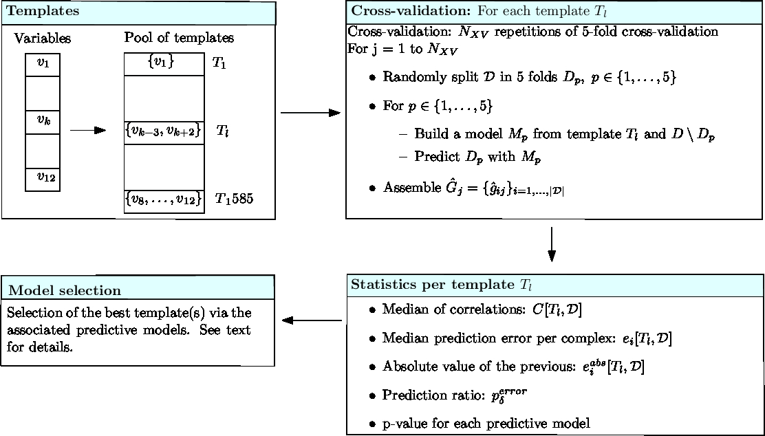
In the sequel, we explain how to predict $\text{\deltagexp}$ of complexes from a dataset $\calD$ , using the methodology summarized on Fig fig-bap-workflow . Estimation is performed on a per complex basis, from which performances at the whole dataset level are derived.

Our predictions rely on three related concepts defined precisely hereafter (see also Fig fig-bap-workflow):

Template: a fixed set of variables from $\calV$ ,
Model: a regression model consisting in a template plus the associated coefficients. As we shall see, such models are associated with cross-validation folds.
Predictive model for $\calD$ : the machinery returning one binding affinity estimate $\hatgi$ per complex from $\calD$ , using $\NXV$ repetitions of the -fold cross validation.

Templates.

Denote $\calV$ the pool of variables. Let a template be a set of variables, i.e. a subset of $\calV$ . To define parsimonious templates from the set $\calV$ , we generate subsets of $\calV$ involving up to at most variables. This defines a pool of templates $\calT = { T_1, \dots, T_{N}}$ .

Cross-validation.

In the following a model is associated to both a template $T_l\in \calT$ and a dataset $\calD$ . More precisely, a model refers to a regression model, i.e. the variables of the template plus the associated coefficients.

Practically, models are defined during -fold cross-validation, and a number of $\NXV$ of repetitions (see Fig fig-bap-workflow). Consider one repetition, which thus consists of splitting at random $\calD$ into subsets called folds. For one fold, a regression model associated with is trained on (k-1)/k of the dataset $\calD$ , and predictions are run on the remaining 1/k of complexes. Processing the folds yields one repetition of the cross validation procedure, resulting in one prediction $\text{\hatgij}$ for the $\text{\deltagexp}$ of each complex. The set of all predictions in one repeat, say the th one, is denoted

Note again that these predictions stem from regression models associated with , namely one per fold.

Statistics per template.

Considering one cross-validation repetition , we define the correlation $\text{\corrj}$ as the correlation between the experimental values ${ \deltagexp }$ and the predictions $\hatGj$ . An overall assessment of the template using the $\NXV$ repetitions is obtained by the following median of correlations

For a complex , we define the binding affinity prediction $\text{\hatgi}$ as the median across repetitions i.e.

The median prediction error is defined by

and the median absolute prediction error by:

Using this latter value, we define the prediction ratio $\pdeltaG{\delta}$ as the percentage of cases such that the dissociation free energy is off by a specified amount $\delta$ :

In particular, setting $\delta$ to 1.4, 2.8 and 4.2 kcal/mol in the previous equation yields cases whose $\Kd$ is approximated within one, two and three orders of magnitude respectively.

Finally, a permutation test yields a p-value for each predictive model [155] .

In a nutshell, the rationale consists of generating randomized datasets by shuffling their $\text{\deltagexp}$ values. Then, one computes the performance criterion for each such dataset, from which the p-value is inferred (see Algorithm~alg-p-val).

Model selection.

Define the best predictive model as the one maximizing performance criterion. We wish to single out the best predictive models, i.e. those that cannot be statistically distinguished from the best predictive model. More precisely, consider a pool of predictive models $\calT$ , out of which we wish to identify a subset of predictive models whose distribution cannot be distinguished from that of the best predictive model. To this end, let H0 be the null hypothesis stating that two predictive models yield identical performance distributions. We decompose the predictive models as $\calT = \calT_1 \cup \calT_2$ such that :

(i) the best predictive model is in $\calT_1$ ,
(ii) in comparing two predictive models from $\calT_1$ , one does not reject H0, and
(iii) in comparing one predictive model from $\calT_1$ against one predictive model from $\calT_2$ , one rejects H0.

The predictive models in $\calT_1$ are called the specific models for the dataset $\calD$ . The corresponding procedure is based on the Kruskal-Wallis test, see [135] .

The p-value threshold for this test is set to $\alpha=0.01$ .

Running binding affinity predictions for a dataset $\calD$ i.e. a subset of the structure affinity benchmark: graphical outline of the statistical methodology.
(Templates) From the pool of variables, templates are generated.

(Cross-validation) Each template undergoes a number $\NXV$ of repetitions of cross-validation, yielding one binding affinity prediction per complex for each repetition.

(Statistics) Various statistics are computed to assess the performances yielded by the predictive model associated to each template.

(Model selection) Predictive models are compared, and the best ones selected.

Input: Specifications and File Types

Model generation and selection is performed by the script $\text{\bapESelect}$ which is executed as follows :

# Quick example: maximum 2-variables models, 10 repetitions and p-value permutations,
# flexible complexes only (irmsd > 1.5 A), run on a single process
sbl-bap-step-3-models-analysis.py -f results/affinity_dataset.xml -m 2 -n 1 -r 10 -p 10  -l 1.5 -o flex_quick

# Heavier example: maximum 4-variables models, 100 repetitions and
# 1000 p-value permutations, all complexes, run on three
# processes. Performs k-nearest neighbors regression with 10 neighbors
sbl-bap-step-3-models-analysis.py -f results/affinity_dataset.xml -m 4 -n 3 -r 100 -p 1000 -k 10 -o all_heavier

The main options of the program

are:
(-f, –data-file-path) string: path to the file resulting from running

(required)
(-m, –max-order) int: maximum order (i.e. number of variables) to be included in a model (required)
(-a, –matching-atoms-filter) float(= 0.8): minimum proportion of atoms matched from a complex structure to its unbound partners structures required for an entry to be included
(-n, -nb-process) int(= 1): number of processes on which to dispatch the execution
(-d, –nb-folds) int(= 5): number of folds of the cross-validation
(-r, –nb-repeats) int(= 1000): number of repetitions of the cross-validation procedure
(-p, –nb-pval-permutations) int(= 1000): number of permutations used to compute the p-value of a model
(-l, –irmsd-lower-bound) float: minimum

allowed for an entry to be included
(-s string(= –filter-file-path)): path to the file giving upper and lower bounds on specific variables from the dataset.
(-i, –inclusive-bounds) bool(= False): set if the previous bounds should be inclusive instead of strict
(-o, –output-file-prefix) string: prefix for the output file
(-k, –knn) bool(= False): toggle knn regression instead of linear regression with the given number of neighbors

The XML file specified by option -f should comply with the following format:

Each entry should be contained in an <entry> element
Each entry should contain the same elements
Each element within an entry should have an attribute type set to one of the following values:
- "info": for general information (e.g. PDB ID, chains, ...) which will not be used during the model selection
- "dep_var": for the dependent variable, i.e. the one to be predicted
- "feature": for the variables to be used during the regression

The txt file specified by option -s should comply with the following format:

Each line contains three non space-containing three elements separated by spaces
The first element is the variable name as specified on the XML data file described above
The second element is the lower bound on the values of the corresponding variable (inclusive if option -i is used)
The third element is the upper bound on the values of the corresponding variable (inclusive if option -i is used)
The character "*" indicates that any value is allowed (e.g. the line "V1 * 1", means an upper bound of value 1 for variable V1)
If a variable name is not in this file, no lower/upper bounds are set

File Name	Description
XML archive file	Compiled data generated from $\text{\bapECompile}$

Input files for the third step described in section Input: Specifications and File Types .

Output: Specifications and File Types

This step outputs a minimum of seven files:

Files 1 and 2 are text files with the following structure:
- A line giving the (0-based) index of the last significantly best model. All models ranked higher are statistically equally good, and all models ranked lower are statistically worse.
- A table with models as rows and various metrics associated (error, correlation, p-values, ...)
In the first one, the index and the ranks are computed on the cross-validated median absolute error of the model. In the second they are computed on the median cross-validation correlation coefficient.
Files 3 and 4 below contain a matrix of prediction per cross-validation repetition for the best model. Here "best" refers to the model selected by the model selection procedure described above. If multiple models are selected, each one has an associated file. These files are structured as follows:
- Each line i corresponds to a sample/entry
- Each column j corresponds to a cross-validation repetition
- A cell i,j contains the value predicted for sample/entry i at repetition j
File 5 and 6: PDF files containing scatter plots of the prediction made by the best predictive models (from files 1 and 2 respectively) for each complex against the experimental affinity value.
File 7: an optional PDF file output only when the $\text{\irmsd}$ is provided. The file contains a scatter plot of the prediction error (Eq. eq-median_error_cplx) made by the best predictive model (correlation-wise) for each complex against its $\text{\irmsd}$ .

Preview	File Name	Description
	Plain text file	File 1
	Plain text file	File 2
	Plain text file	File 3
	Plain text file	File 4
	PDF file	Scatter plot of the prediction versus experimental affinity for the best model(s)
	PDF file	Scatter plot of the prediction versus experimental affinity for the best model(s)
	PDF file	Scatter plot of the prediction error versus interface RMSD

Output files for the step 3 described in section Input: Specifications and File Types

Model exploitation: predicting affinities

Once a set of variable has been selected during the previous step, it can be used to estimate a model. Recall that a model is a function returning an estimate for binding affinity of a complex. For this, one needs a training set and a regressor, i.e. an object able to use the training set to predict the affinity of a new dataset (for instance, linear least-squares fitting, nearest neighbors, regression trees, ...). An example of the procedure to train such a regressor on the whole Structure Affinity Benchmark and predict its own entries (that is to perform predictions without cross-validation) is given in a demo file (sbl-binding-affinity-model-exploitation-example.py).

Algorithms and Methods

We now describe two algorithms used by this package. The first simply computes an approximate (upper bound on the) permutation p-value for a given statistic [155] . The pseudo-code is given on Algorithm alg-p-val .

The second algorithm is used to divide a pool of models into two groups, namely $\calT = \calT_1 \cup \calT_2$ , as discussed in the section Using the programs to select affinity prediction models . The corresponding procedure is based on the Kruskal-Wallis test, and can be found in [135] .

$\begin{algorithm}\begin{algorithmic} \Require{$\calD$: dataset; $T_l$: a template; $p_{T_l}$: a performance criterion for $Tx_l$; $\Nperm$: number of repetitions} \For{ $q \in \{1 \dots \Nperm\}$} \State{Randomly permute the dependent variable in $\calD$ (here the affinity) to obtain $\calD^{perm}_q$} \State{Perform 5-fold cross-validation of regression models using the variables in $T_l$ on $\calD^{perm}_q$} \State{Store the performance criterion in $p^{perm}_{T_l}$} \EndFor \State Report the approximate p-value for $T_l$ to be $\frac{B+1}{\Nperm + 1}$, with $B$ the number of elements in $p^{perm}_{T_l}$ which are more extreme than $p_{T_l}$. \end{algorithmic} \caption{{\bf Computing a permutation p-value for a binding affinity predictive model specified by a template $T_l$.} The p-value is based on a permutation test, which uses the prediction performances obtained on random datasets, each such dataset being obtained by permuting the dependent variable (i.e. the affinity) over the dataset.} \end{algorithm}$

Programmer's Workflow

Pre-processing

We describe successively the 2 steps of section Using the programs to pre-process structural data .

Step 1.

The script $\text{\bapERun}$ runs applications from the SBL on the bound and unbound partners.

The matching between atoms (section Matchings for atoms) is done using the python module SBL::PDB_complex_to_unbound_partners_matchings which is a wrapper around the executable $\text{\alignPDBRA}$ . This executable performs the matching using the class SBL::CSB::T_Alignment_engine_sequences_seqan, from the package Alignment_engines, which itself uses the Seqan library to perform the sequence alignment, and subsequently match residue and atoms based on the alignment found.

In order to compute shelling orders and packing properties, the executables $\text{\sblvorlumepdb}$ and $\text{\sblvorshellE}$ are also run on the complex, and $\text{\sblvorlumepdb}$ is run on the unbound partners.

Step 2.

The script $\text{\bapECompile}$ compiles the previous results and computes the variables listed in section Associated variables for each entry of the dataset.

Data structures to store the properties of entities such as atoms, residues, chains and files are grouped in the python module SBL::Protein_complex_analysis_molecular_data_structures . To fill these data structures it also provides a class used to traverse the directory structure and parse the files resulting from step 1.

Model selection

The machinery used to build, evaluate and rank various models using the previously computed variables can be found in the python module SBL::Combinations_of_variables_model_evaluation::Combinations_of_variables_model_evaluation .

Model exploitation

Once a set of variables has been selected, model fitting on a training set and prediction of a new dataset can be done using any software or language. An example script is given using python and scikit-learn in file $\text{\bapESelect}$

External dependencies

The seqan library [76] (BSD, Seqan) is necessary when computing the variables which encode the variations between bound and unbound partners.