|
Structural Bioinformatics Library
Template C++ / Python API for developping structural bioinformatics applications.
|
|
Structural Bioinformatics Library
Template C++ / Python API for developping structural bioinformatics applications.
|
Authors: F. Cazals and T. Dreyfus
![]()
We consider a structure (molecule, complex) decomposed into units. A unit may be a polypeptide chain, a domain, a set of residues, etc. Our focus is on interactions between these units, and we ascribe such interactions to two categories, referred to as geometric interactions/interfaces and biochemical interactions/interfaces.
Geometric interactions/interfaces. Such interfaces typically correspond to non-covalent interactions between atoms ascribed to units. Typical cases where such interfaces are of interest are:
For each geometric interface between two units, high level information is provided, including (i) the number of particles involved at each interface, (ii) tThe number of connected components i.e. patches of each interface. These pieces of information provide a first indication on the various contacts between the molecules in presence, e.g. to select interfaces to further investigate using the applications of Space_filling_model_interface from Space_filling_model_interface .
Biochemical interactions/interfaces. The focus here is on more local interactions between units, such as disulfide bonds and ionic interactions–see the package Pointwise_interactions.
Applications provided. The applications 

Contacts. Consider a model in a PDB file, consisting of chains made of particles. We assume (details below), that each particle has been assigned a primitive label, as defined in the concept MolecularSystemLabelsTraits. For the program
Consider the 
Our focus is on contacts, which are of two types, bicolor and mediated. In the sequel, we briefly recall the definitions of these concepts, and refer the reader to the package Space_filling_model_interface for more details.
An edge in the alpha complex defines a bicolor contact provided that its endpoints carry two different primitive labels. To define a mediated contact, consider a mediator particle sandwiched between two particles with different primitive labels (i.e, there is an edge from both partners' particles to the mediator's particle). Such a particle induces two mediated contacts, one with each particle carrying a primitive label – see Fig. fig-bif-mediated-contact.
Interfaces. The contacts between partners are edges of the
The program
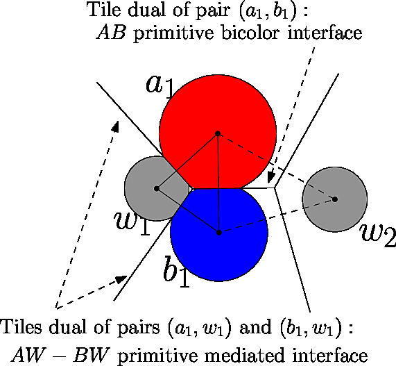 |
Voronoi interfaces: bicolor and mediated. This fictitious molecular structure involves two partners A (red) and B (blue) and two water molecules (gray). A and B make one bicolor contact; the water molecule |
This packages hinges on the functionalities from the package Tertiary_quaternary_structure_annotator, so as to report a number of specific interactions between regions in a structure or complex, such as:
This section presents the program
Input. A PDB file. Note that
Main options.
Note that a default radius of 
Main output. Main output files:
Remarks.
This section presents the program
Input. Running
Main options.
Main output.
Comments.
The SBL provides VMD, PyMOL, and Web plugins for sbl-bif-chainW-atomic.exe. Launch the VMD plugin from the SBL catalog under the Extensions menu, start the PyMOL plugin by running sbl_bif_chainW_atomic in the PyMOL command line, and open the Web plugin from the SBL web plugins launcher page (served locally via sbl-web-plugins-launcher). All three plugins expose the same GUI and capabilities.
 |
sbl-bif-chainW-atomic plugin user interface. The user interface for the sbl-bif-chainW-atomic plugin. The typical workflow is: Step 1: Load a molecular structure from a PDB file. Step 2: Choose an output directory (optional, a default is provided). Step 3: Launch the computation. Step 4: Inspect the results in the viewer. Step 5: Review the calculation statistics and interface graphs in the GUI. |
Using the notions of bicolor and mediated contacts recalled in the section Prerequisites, assume that
The applications perform two tasks:
See algorithms in the package Pointwise_interactions.
The programs of Space_filling_model_interface_finder described above are based upon generic C++ classes, so that additional versions can easily be developed for protein or nucleic acids, both at atomic or coarse-grain resolution.
In order to derive such versions, there are two important ingredients, that are the workflow class, and its traits class.
T_Space_filling_model_interface_finder_traits:
T_Space_filling_model_interface_finder_workflow:
In the sequel, we study two cases:
#!/usr/bin/python

import re  #regular expressions
import sys #misc system
import os
import pdb
import shutil # python 3 only


def find_file_in_output_directory(str, odir):
    cmd = "find %s -name *%s" % (odir,str)
    return os.popen(cmd).readlines()[0].rstrip()

def run_calculation(pdbid):
    #input filename  and output directory
    pdb_prefix = pdbid.rsplit(".")[0]
    ifname = "../../../demos/data/%s" % pdbid
    odir = "results-%s" % pdb_prefix
    if not os.path.exists(odir): os.system( ("mkdir %s" % odir) )

    # check executable exists and is visible
    exe = shutil.which("sbl-bif-chainsW-atomic.exe")
    print( ("Using executable %s\n" % exe) )

    # run command
    cmd = "%s -f %s -p 1 --directory %s --verbose --output-prefix --log" % (exe,ifname,odir)
    os.system(cmd)

    # list output files
    ofnames = os.popen( ("ls %s" % odir) ).readlines()
    print("\nAll output files are:",ofnames)

    # find the lof file and display log file
    lfname = find_file_in_output_directory("log.txt", odir)
    print("\nLog file is:", lfname)
    #log = open(lfname).readlines()
    # for line in log:         print(line.rstrip())

run_calculation("1vfb.pdb")
The 1vfb file contains three polypeptide chains names A, B, and C.
from IPython.display import Image

def display_graphs(pdbid):
    pdb_prefix = pdbid.rsplit(".")[0]
    ifname = "../../../demos/data/%s" % pdbid
    odir = "results-%s" % pdb_prefix

    # find the dot file listing interfaces
    of_interf_dot = find_file_in_output_directory("vor_interfaces_graph.dot", odir)
    of_interf_xml = find_file_in_output_directory("vor_interfaces_graph.xml", odir)


    # plot and display image
    of_geom_png = "%s-geom_interfaces.png" % pdb_prefix
    cmd = "dot -Tpng %s -o %s" % (of_interf_dot,of_geom_png);  os.system(cmd)

    print("Interfaces within chains of   PDB file:")
    img_geom = Image(filename = of_geom_png, width=300, height=300);  display(img_geom)

    # likewise for biochemical interfaces i.e. S-S bonds and salt bridges
    of_biochem_dot = find_file_in_output_directory("biochemical_interfaces_graph.dot", odir)
    of_biochem_xml =  find_file_in_output_directory("biochemical_interfaces_graph.xml", odir)


    # plot and display image
    of_biochem_png = "%s-biochem_interfaces.png" % pdb_prefix
    cmd = "dot -Tpng %s -o %s" % (of_biochem_dot, of_biochem_png);     os.system(cmd)

    print("S-S bonds and salt bridges within PDB file:")
    img_biochem = Image(filename = of_biochem_png, width=300, height=300); display(img_biochem)


display_graphs("1vfb.pdb")


For the graph of interfaces:
For the graph of S-S bonds and salt bridges: no relevant information here.
The following example is quite interesting: as a complete immunoglobulin, we investigate the contacts between the four chains, from a geometric standpoint as well as in terms of S-S bonds and salt bridges
run_calculation("1igt.pdb")
display_graphs("1igt.pdb")


The graph of interfaces illustrates the contacts between the heavy and light chains of the IG.
The graph of S-S bonds illustrates disulfide bonds found across the chains. S-S bonds within a chain can also be reported with the option --internal, as illustrated below.
(left) The structure involves four chains. Note in particular the 3 disulfides bonds connecting the two heavy chains (right) The graph produced, with edges counting disulfide bonds and salt bridges. Note that there is a total of 17 / 17 S-S bonds and 18 salt bridges.
display(Image(filename ="fig/1igt-biochem-annotations--montage.png", width=500, height=500));

This more complex example involves 16 subunits.
run_calculation("4D10.pdb")
display_graphs("4D10.pdb")


As can be seen, there are many more interfaces and biochemical features of interest. A full description of the findinds is reported in the xml files dumped into the results directory. Such files should be parsed with PALSE, see https://sbl.inria.fr/doc/PALSE-user-manual.html
Recall that class II fusogens act as trimers. Assume that a decomposition of a monomer into domains has been provided using labels. All contacts between such domains are easily infered.
#input filename  and output directory
pdbid = "4ojc--EFF1-trimer.pdb"
pdb_prefix = pdbid.rsplit(".")[0]
ifname = "../../../demos/data/4ojc--EFF1-trimer.pdb"
domain_labels = "../../../demos/data/4ojc--EFF1-trimer-partners.txt"

odir = "results-%s" % pdb_prefix
if not os.path.exists(odir): os.system( ("mkdir %s" % odir) )

# check executable exists and is visible
exe = shutil.which("sbl-bif-domainsW-atomic.exe")
print( ("Using executable %s\n" % exe) )

# run command
cmd = "%s -f %s --domain-labels  %s --directory %s --verbose --output-prefix --log"\
    % (exe, ifname,domain_labels, odir)
print("Running ",cmd)
os.system(cmd)
display_graphs("4ojc--EFF1-trimer.pdb")


As for the previous example, an automatic processing of the xml files delivered is in order.
