Structural Bioinformatics Library
Template C++ / Python API for developping structural bioinformatics applications.
User Manual

Authors: F. Cazals and T. Dreyfus and C. Roth

Energy_landscape_analysis

This package provides various methods to analyze sampled energy landscapes, with in particular various statistics on its transition and connectivity graphs.

Goals

We have seen in the package Transition_graph_of_energy_landscape_builders that there are three options to build a transition graph (see def. def-transition-graph):

  • from a database of stationary points,
  • from a collection of pairs (sample, associated local minimum),
  • from a collection of samples.

In the following, we exploit such transition graphs, to ultimately gain insights on the structure and dynamics of molecular systems, see [173] and [67] . In this perspective, this package proposes various methods to characterize sampled energy landscapes.

The following functionalities are provided on transition graphs and disconnectivity graphs (see def. def-DG):

  • Transition graph

    • topological properties (Betti Numbers) ,
    • metric properties i.e. path lengths.

  • Transition graph: Morse based analysis, including persistence analysis for local minima and distribution of barriers' heights.

  • Disconnectivity graphs: computation of morphological properties (internal path length),

These functionalities are available in the programs $\sblELAL$ and $\sblELAE$.

Prerequisites

Transition graphs: topology and Betti Numbers

A variety of algorithms can be used to explore energy landscapes, and their results can be turned into a compressed transition graph – definition def-transition-graph, using e.g. methods presented in the package Transition_graph_of_energy_landscape_builders.

In the sequel, we are interested in topological and geometric information characterizing such graphs.

Topological information. For a given graph, the number of connected components and the number of cycles in this graph are known as the first and second Betti numbers [79] , and are respectively denoted $\beta_0$ and $\beta_1$. We report them for the transition graph, and we also compute statistics on a per connected component basis.

The presence of cycles in a transition graph is especially interesting, since such cycles correspond to different paths connecting the same local minima. Cycles involving two edges are also of interest, as they may arise in two situations. The first corresponds to the situation in which a loop around a saddle is anchored in a single local minimum (Fig. fig-bump-middle-slope-bassin). The second is due to post-sampling processing techniques that may be used to group minima. For instance, in the BLN model, enantiomeric left and right handed helices may be considered as identical in certain contexts; identifying them as such results in the creation of a cycle.

Geometric information. Assume a distance $\dCalC$ between conformation has been chosen. The simplest geometric information embodied in a transition graph is the length of its edges, and can be assessed with the statistical summary of Eq. (eq-stat-triple-edge-lengths).

In particular, the presence of long edges hints at challenging landscapes: even when the $\dCalC$ between all pairs of local minima is small, one may have to follow a long valley to reach a saddle connecting two minima.

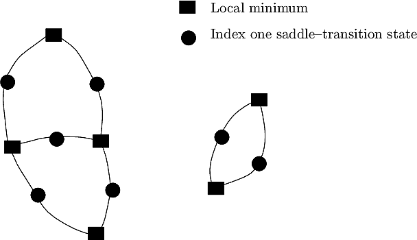
Describing the topology of a transition graph with the first and second Betti numbers
This fictitious examples features a TG with two connected components: the first one involves four local minima and five saddles; the second one involves two local minima and two saddles. The Betti numbers are:
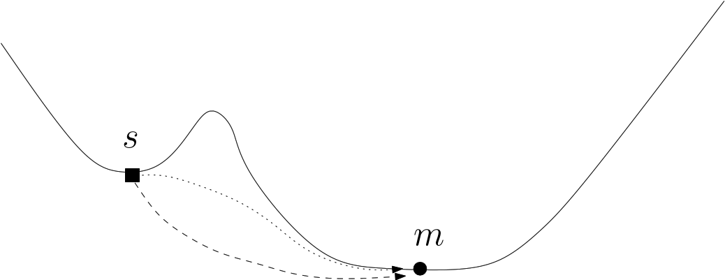
 $\beta_0=2$ (two connected components) and $\beta_1=3$ (three cycles).

A loop around a saddle $s$ may be anchored in a single local minimum $m$ — a.k.a bump transition
Note that the dotted path is located behind the bump of this fictitious 2D landscape.

Transition graphs: paths from minima to saddles

Consider a transition graph, and assume that selected minima called landmarks have been singled out. For example, one may select the lowest local minima or the most persistent ones (package Morse_theory_based_analyzer).

For a given landmark, the distribution of distances from that landmark to its connected saddles provides an estimate on the size of the basin of that landmark [74] . Also, a large value for the smallest such distance provides information on the distance to be traveled to escape from the basin of that minimum. Similarly, the relative position of all landmarks is assessed by the statistical summary of all pairwise distances.

The shortest route between two landmarks is not always the easiest one, as in particular it may pass through steep sections of the landscape. We therefore offer the possibility to filter out a TG in several ways, before computing the statistics just defined
  • by removing vertices above a certain height
  • by removing edges whose gradient magnitude is beyond a certain threshold.


Morse based analysis

Morse theory and topological persistence provide a number of concepts and tools which are highly relevant to study energy landscapes. We describe a few of them in the sequel, and refer the reader to the terminology section Terminology and Concepts for a quick recap on central notions such as sublevel set, key saddle, Morse-Smale-Witten complex.

Of particular interest is the pairing between local minima and their key saddles (see def. def-key-saddle). This pairing, and more specifically the elevation drop between the key saddle and its minimum indeed defines the barrier height. The elevation of the minimum of that of its key saddle may also be seen as the birth date and the death date of the catchment basin of the local minimum: when scanning the landscape with a horizontal plane, the basin appears at the elevation of the local minimum, and disappears i.e. merges with another basin at the elevation of its key saddle. Putting together all points (birth date, death date) defines the so-called persistence diagram (PD), as detailed in the package Morse_theory_based_analyzer.

Persistence diagrams for sublevel sets. The analysis presented above for local maxima and super level sets applies directly for local minima and sublevel sets, yielding a persistence diagram whose points code local minima of the height field. The executive summary concerning the PD of a landscape goes as follows:

  • By construction, the lowest local minimum is not paired with any saddle. That is, if the height field has $m$ local minima, its PD contains $m-1$ points.

  • A point of the PD corresponds to a pairing involving one local minimum and one saddle. Mathematically, these points are critical points of the height field: the minimum is an index $0$ c.p. (its Hessian has zero negative eigenvalues), while the saddle is an index one c.p. (its Hessian has one negative eigenvalue).

  • All points of the PD are above the diagonal $y=x$, and the distance from a point to the diagonal is a measure of the stability of the corresponding local minimum.

  • A PD can also be simplified by re-assigning the basins of non significant minima. That is, if the points of the PD are clearly separated, those near the diagonal can be removed by merging each such basin into the deeper basin it is connected to. Note that this simplification removes the least persistent basins first, as opposed to merging the saddles in a given energy slice. Note also that this simplification cancels one (saddle, minimum) pair at a time.
As discussed in the package Morse_theory_based_analyzer , Morse theory based analysis can be conducted in two rather different settings, namely by considering a graph connecting sample points, or a graph connecting critical points. The reader is referred to section Graph connecting sample points versus graph connecting critical points for more details on these two options. Also check the –skip-saddle-SM option of the applications in this package.


Disconnectivity graphs: morphology

The disconnectivity graph (DG) of a landscape describes the merge events of catchment basins, which occur at key saddles (see also def. def-DG).

The generic situation expected in a DG is that of a binary merge, namely a saddle is linked to two local minima. (Degenerate situations may occur, though: for example, a monkey saddle is linked to three local minima.) That is a generic DG is a binary tree: each internal node representing a saddle is associated with at most two children, and each leaf represents a local minimum.

The morphology of a complete binary tree can vary between that of a path (in which one child of each internal node is a leaf and the other is an internal node) and that of a perfectly balanced tree (in which each internal node has two children i.e. subtrees of the same size). To assess the structure of such trees, we use the so-called external path length (EPL) [122] . Defining the depth of a node as the number of edges required to reach it from the root, the EPL is the sum of depths of the leaves of the tree. Likewise, the internal path length (IPL) is the sum of the depth of internal nodes. If $n$ is the number of internal nodes (index one saddles in our case), the EPL when the tree is a path is $\binom{n}{2}+2n$, which we will write using the shorthand $\eplPath$, while that of a perfectly balanced tree is $n\log_2 n$. Since the latter, symmetrical tree is not a realistic reference, we use instead the EPL of a random binary search tree [122] , which is asymptotically equivalent to $\eplRand \sim 2n\ln n$.

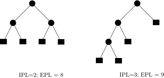
Internal and external path lengths of binary trees (IPL and EPL)
The IPL counts the number of edges traversed, from the root, to reach internal nodes (disks); in the context of disconnectivity graphs for energy landscapes, recall that these refer to key saddles. The EPL counts the number of edges traversed to reach the leaves of the tree; in the context of DG, these refer to local minima.

Using sbl-energy-landscape-analysis-euclid.exe

Main specifications

Main options.

The main options of the program $\sblELAE$ are:
–transition-graph string: xml file representing the compressed transition graph of a sampled energy landscape
–topology: run topology analysis over the uncompressed transition graph
–Morse: run Morse theory based analysis over the uncompressed transition graph with the potential energy as Morse function
–skip-saddle-SM: When performing persistence based simplification, do not report the stable manifold of saddle points
–landmarks: run shortest paths analysis through input landmark vertices on the compressed transition graph
–landmarks-filename string: file listing the landmark indices in the compressed transition graph


Input.

The main input is a transition graph of a sampled energy landscape, produced by the programs of the application Transition_graph_of_energy_landscape_builders as XML archives. If shortest paths with landmarks are desired, it is required to load a file listing the vertices of the input transition graph that are the landmarks. A strategy for producing a landmarks file consists on comparing the input transition graph with a reference transition graph containing only reference conformations. Programs of the application Energy_landscape_comparison produce a Graphviz file showing the correspondence between the vertices of two input transition graphs. This allows to visually select the vertices of an input graph that will be landmarks.

  • (xml format, suffix transition_graph.xml) Landmarks file: –landmarks-filename data/bln69_transition_graph.xml

Main output.

Identical to those obtained when building the transition graph see Main specifications, yet possibly corresponding to a different persistence threshold:

  • (txt format, suffix log.txt) Main log file
  • (eps format, sufix , suffix disconnectivity_forest.eps) Disconnectivity forest in eps file format.
  • (xml format, suffix stable_manifold_partition.xml) Stable manifold partition: XML archive listing the samples repartition by persistent basin of the landscape. The first sample listed for a basin is the local minimum.
  • (txt format, txt file, suffix cluster_leaders.txt) Cluster leaders: the index of the leading point associated to a basin.
  • (txt format, suffix persistence_diagram.txt) Persistence diagram, list of all basins sorted by persistence. Nb: by convention, the persistence of the global minimum of a connected component is reported as:
    index (integer) inf (keyword) elevation (floating point number)
    
  • (txt format, suffix persistence_histogram.txt)
    Persistences: list of all finite persistences.
  • (pdf format, suffix persistence_histogram.pdf) Persistence histogram: pdf format, drawn by R.
  • (xml format, suffix MSW_chain_complex.xml) Morse Smale Witten chain complex, which connects critical points in codimension one, serialized using Boost into an XML archive.

Optional output.

Using sbl-energy-landscape-analysis-lrmsd.exe

Main specifications

Main options.

The main options of the program $\sblELAL$ are:
–transition-graph string: xml file representing the compressed transition graph of a sampled energy landscape
–topology: run topology analysis over the uncompressed transition graph
–Morse: run Morse theory based analysis over the uncompressed transition graph with the potential energy as Morse function
–skip-saddle-SM: When performing persistence based simplification, do not report the stable manifold of saddle points


Input. See section above.

Main output. See section above.

Algorithms and Methods

Transition graphs: topology and Betti Numbers

Computing the first and second Betti number of a graph respectively require running a traversal of the graph and a union-find algorithm [79], [61] .

The classical construction of a transition graphs resorts to transition path sampling algorithms to connect local minima. We offer an alternative calculation merely requiring a set of samples and their quenched counterparts, based on a variant of the algorithm explained in section Morse based analysis .


Transition graphs: paths

Computing the distances between landmarks can be done using a variant of Dijkstra's shortest path algorithm, where one walks on the graph provided, but records and relaxes distances between landmarks only [61] .

To compute statistics on a filtered graph one applies Dijkstra's (or its variant with landmark), on a filtered graph which is the graph induced by the vertices which have not been filtered out on the height criterion, and where selected edges have possibly been removed.


Programmer's Workflow

The programs of Energy_landscape_analysis described above are based upon generic C++ classes, so that additional versions can easily be developed.

In order to derive other versions, there are two important ingredients, that are the workflow class, and its traits class.

The Traits Class

T_Energy_landscape_analysis_traits:

The Workflow Class

T_Energy_landscape_analysis_interface_workflow:

Other Utilities

This package provides also the program sbl-energy-landscape-analysis-graph-star.exe, allowing to select/extract/perform statistics on the star of a vertex in a weighted graph.

Jupyter demo

See the following jupyter notebook:

  • Jupyter notebook file
  • Energy_landscape_analysis

    Energy_landscape_analysis

    Transition graphs of energy landscapes

    We have seen in the package Transition_graph_of_energy_landscape_builders that there are three options to build a transitio graph:

    • from a database of stationary points
    • from a collection of pairs (sample, associated local minimum)
    • from a collection of samples.

    In the following, we exploit such transition, as explained in the User manual.

    Useful functions

    In [1]:
    from SBL import SBL_pytools
    from SBL_pytools import SBL_pytools as sblpyt
    help(sblpyt)
    
    Help on class SBL_pytools in module SBL_pytools:
    
    class SBL_pytools(builtins.object)
     |  Static methods defined here:
     |  
     |  convert_eps_to_png(ifname, osize)
     |  
     |  convert_pdf_to_png(ifname, osize)
     |  
     |  find_and_convert(suffix, odir, osize)
     |      # find file with suffix, convert, and return image file
     |  
     |  find_and_show_images(suffix, odir, osize)
     |  
     |  find_file_in_output_directory(suffix, odir)
     |  
     |  show_eps_file(eps_file, osize)
     |  
     |  show_image(img)
     |  
     |  show_log_file(odir)
     |  
     |  show_pdf_file(pdf_file)
     |  
     |  show_row_n_images(images, size)
     |  
     |  show_text_file(file_suffix, odir)
     |  
     |  show_txt_file(file_suffix, odir)
     |  
     |  ----------------------------------------------------------------------
     |  Data descriptors defined here:
     |  
     |  __dict__
     |      dictionary for instance variables (if defined)
     |  
     |  __weakref__
     |      list of weak references to the object (if defined)


    Running the executables: main options

    The options of the analyze method in the next cell are:

    • metric: euclid or lrmsd
    • transGraph: xml file representing the compressed transition graph of a sampled energy landscape
    • landmarks: run shortest paths analysis through landmark vertices on the compressed transition graph listed on an input text file
    • topology: run topology analysis over the uncompressed transition graph
    • Morse: run Morse theory based analysis over the uncompressed transition graph with the potential energy as Morse function
    In [2]:
    import re  #regular expressions
    import sys #misc system
    import os
    import pdb
    import shutil # python 3 only
    from IPython.display import Image
    from IPython.display import IFrame
    
    
    def analyze_transition_graph(metric, transGraph, landmarks = None, topology = True, Morse = True):
    
        odir = "tmp-results-%s" % metric
        if os.path.exists(odir):
            os.system("rm -rf %s" % odir)
        os.system( ("mkdir %s" % odir) )
        
        # check executable exists and is visible
        exe = shutil.which("sbl-energy-landscape-analysis-%s.exe" % metric)
        if not exe: 
            print("Executable not found")
            return 
        
       
        print(("Using executable %s\n" % exe))
        cmd = "sbl-energy-landscape-analysis-%s.exe --transition-graph %s \
                  --directory %s --verbose --log " % (metric, transGraph, odir)
        if landmarks:
            cmd += "--landmarks --landmarks-filename %s " % landmarks
        if topology:
            cmd += "--topology "
        if Morse:
            cmd += "--Morse "
             
        print(("Executing %s\n" % cmd))   
        os.system(cmd)
            
        cmd = "ls %s" % odir
        ofnames = os.popen(cmd).readlines()
        print(("All output files in %s:" % odir),ofnames,"\n")
            
        sblpyt.show_log_file(odir)


    Example 1: the Himmelblau terrain z=f(x,y)

    The Himmelblau function is defined by the bivariate polynomial $f(x,y) = (x^2+y-11)^2 + (x+y^2-7)^2$.

    In [3]:
    from IPython.display import Image
    Image(filename='fig/himmelblau-matlab-cropped.png')
    
    Out[3]:
    In [4]:
    print("Marker : Calculation Started")
    analyze_transition_graph("euclid", "data/himmelbleau_tg.xml", landmarks = "data/himmelbleau_landmarks.txt")       
    print("Marker : Calculation Ended")
    
    Marker : Calculation Started
    Using executable /user/fcazals/home/projects/proj-soft/sbl-install/bin/sbl-energy-landscape-analysis-euclid.exe
    
    Executing sbl-energy-landscape-analysis-euclid.exe --transition-graph data/himmelbleau_tg.xml               --directory tmp-results-euclid --verbose --log --landmarks --landmarks-filename data/himmelbleau_landmarks.txt --topology --Morse 
    
    All output files in tmp-results-euclid: ['sbl-energy-landscape-analysis-euclid__disconnectivity_forest.eps\n', 'sbl-energy-landscape-analysis-euclid__landmarks_paths.xml\n', 'sbl-energy-landscape-analysis-euclid__log.txt\n', 'sbl-energy-landscape-analysis-euclid__MSW_chain_complex.xml\n', 'sbl-energy-landscape-analysis-euclid__persistence_diagram.pdf\n', 'sbl-energy-landscape-analysis-euclid__persistence_diagram.plot\n', 'sbl-energy-landscape-analysis-euclid__persistence_diagram.txt\n', 'sbl-energy-landscape-analysis-euclid__persistence_histogram.pdf\n', 'sbl-energy-landscape-analysis-euclid__persistence_histogram.r\n', 'sbl-energy-landscape-analysis-euclid__persistence_histogram.txt\n', 'sbl-energy-landscape-analysis-euclid__stable_manifold_clusters.txt\n', 'sbl-energy-landscape-analysis-euclid__stable_manifold_partition.xml\n', 'sbl-energy-landscape-analysis-euclid__topology.xml\n'] 
    
    Showing file tmp-results-euclid/sbl-energy-landscape-analysis-euclid__log.txt
    
    ++Showing file tmp-results-euclid/sbl-energy-landscape-analysis-euclid__log.txt
    Running:  sbl-energy-landscape-analysis-euclid.exe --transition-graph data/himmelbleau_tg.xml --directory tmp-results-euclid --verbose --log --landmarks --landmarks-filename data/himmelbleau_landmarks.txt --topology --Morse
    
    Transition Graph Loader
    Statistics:
    
    Persistence Based Topographical Analysis
    Statistics:
    Number of critical vertices of index 0: 4
    Number of regular critical vertices of index 1: 6
    Number of degenerated critical vertices (num, #faces):
    Number of connected components, i.e Betti_0: 1
    Size of connected components (num, size): (1, 10)
    Number of cycles (after simplification), i.e Betti_1: 3
    Number of clusters for stable manifold partition: 4
    Size of stable manifolds, i.e Watershed (num, size): (1, 1) (1, 2) (1, 3) (1, 4)
    
    Report...
    
    Landmark Paths Analysis
    Computing the edge weights...
    
    0%   10   20   30   40   50   60   70   80   90   100%
    |----|----|----|----|----|----|----|----|----|----|
    ***************************************************
    Loading the landmark's indices...
    Computing the shortest paths with landmarks...
    Computing for the 1th landmark...
    Storing the shortest paths to the 1th landmark...
    Computing for the 2th landmark...
    Storing the shortest paths to the 2th landmark...
    Computing for the 3th landmark...
    Storing the shortest paths to the 3th landmark...
    Statistics:
    Transition Graph Landmark Paths statistics...
    Path from 0 to 1: distance: 3.985753, length: 1
    Path from 0 to 3: distance: 8.345440, length: 1
    Path from 1 to 3: distance: 7.273507, length: 1
    Distances min / median / max: 3.985753 7.273507 8.345440
    
    Report...
    
    Topological Analysis
    Computing the distances...
    
    0%   10   20   30   40   50   60   70   80   90   100%
    |----|----|----|----|----|----|----|----|----|----|
    ***************************************************
    Sorting the distances...
    Computing number of connected components and cycles...
    Statistics:
    Transition Graph topology and paths statistics...
    Number of vertices: 4
    Number of edges: 6
    Number of edges per vertex (min, median, mean, max): 3 3 3.000000 3
    Weights over vertices (min, median, mean, max): 0.231200 0.258200 0.248000 0.262900
    Number of connected components: 1
    Number of cycles: 3
    Number of loops over one minimum: 0
    Number of minima with loops: 0
    Number of loops over one minimum in largest connected component: 0
    Distances between samples (min / median / max): 3.985753 7.273507 8.345440
    
    Report...
    
    End Run
    
    General Statistics:
    
    Times elapsed for computations (in seconds):
    -- Topological Analysis: 0.000144
    -- Landmark Paths Analysis: 0.000170
    -- Persistence Based Topographical Analysis: 0.002458
    Total: 0.002772
    
    --Done
    
    
    Marker : Calculation Ended
    
    In [5]:
    ## We can now easily visualize the main plots i.e. the disconnectivity forest and the persistence diagram
    
    In [6]:
    odir = "tmp-results-euclid"
    
    images = []
    images.append( sblpyt.find_and_convert("disconnectivity_forest.eps", odir, 100) )
    images.append( sblpyt.find_and_convert("persistence_diagram.pdf", odir, 100) )
    sblpyt.show_row_n_images(images, 100)
    
    Figs displayed
    

    Example 2: BLN69

    Recall that BLN69 is a toy protein model made of 69 pseudo-amino acids which are either hydrophoBic, hydrophiLic,or Neutral:

    In [7]:
    from IPython.display import Image
    Image(filename='fig/bln69-visu7305.jpg')
    
    Out[7]:

    We first launch the calculation

    In [8]:
    print("Marker : Calculation Started")
    #analyze("euclid", "data/bln69_transition_graph.xml", landmarks = "data/bln69_transition_graph.xml") 
    analyze_transition_graph("lrmsd", "data/bln69_transition_graph.xml", landmarks = "data/bln69_landmarks.txt")      
    print("Marker : Calculation Ended")
    
    Marker : Calculation Started
    Using executable /user/fcazals/home/projects/proj-soft/sbl-install/bin/sbl-energy-landscape-analysis-lrmsd.exe
    
    Executing sbl-energy-landscape-analysis-lrmsd.exe --transition-graph data/bln69_transition_graph.xml               --directory tmp-results-lrmsd --verbose --log --landmarks --landmarks-filename data/bln69_landmarks.txt --topology --Morse 
    
    All output files in tmp-results-lrmsd: ['sbl-energy-landscape-analysis-lrmsd__disconnectivity_forest.eps\n', 'sbl-energy-landscape-analysis-lrmsd__landmarks_paths.xml\n', 'sbl-energy-landscape-analysis-lrmsd__log.txt\n', 'sbl-energy-landscape-analysis-lrmsd__MSW_chain_complex.xml\n', 'sbl-energy-landscape-analysis-lrmsd__persistence_diagram.pdf\n', 'sbl-energy-landscape-analysis-lrmsd__persistence_diagram.plot\n', 'sbl-energy-landscape-analysis-lrmsd__persistence_diagram.txt\n', 'sbl-energy-landscape-analysis-lrmsd__persistence_histogram.pdf\n', 'sbl-energy-landscape-analysis-lrmsd__persistence_histogram.r\n', 'sbl-energy-landscape-analysis-lrmsd__persistence_histogram.txt\n', 'sbl-energy-landscape-analysis-lrmsd__stable_manifold_clusters.txt\n', 'sbl-energy-landscape-analysis-lrmsd__stable_manifold_partition.xml\n', 'sbl-energy-landscape-analysis-lrmsd__topology.xml\n'] 
    
    Showing file tmp-results-lrmsd/sbl-energy-landscape-analysis-lrmsd__log.txt
    
    ++Showing file tmp-results-lrmsd/sbl-energy-landscape-analysis-lrmsd__log.txt
    Running:  sbl-energy-landscape-analysis-lrmsd.exe --transition-graph data/bln69_transition_graph.xml --directory tmp-results-lrmsd --verbose --log --landmarks --landmarks-filename data/bln69_landmarks.txt --topology --Morse
    
    Transition Graph Loader
    Statistics:
    
    Persistence Based Topographical Analysis
    Statistics:
    Number of critical vertices of index 0: 100
    Number of regular critical vertices of index 1: 168
    Number of degenerated critical vertices (num, #faces):
    Number of connected components, i.e Betti_0: 1
    Size of connected components (num, size): (1, 327)
    Number of cycles (after simplification), i.e Betti_1: 69
    Number of clusters for stable manifold partition: 100
    Size of stable manifolds, i.e Watershed (num, size): (4, 1) (37, 2) (32, 3) (15, 4) (2, 5) (1, 6) (4, 7) (2, 8) (2, 10) (1, 13)
    
    Report...
    
    Landmark Paths Analysis
    Computing the edge weights...
    
    0%   10   20   30   40   50   60   70   80   90   100%
    |----|----|----|----|----|----|----|----|----|----|
    ***************************************************
    Loading the landmark's indices...
    Computing the shortest paths with landmarks...
    Computing for the 1th landmark...
    Storing the shortest paths to the 1th landmark...
    Computing for the 2th landmark...
    Storing the shortest paths to the 2th landmark...
    Statistics:
    Transition Graph Landmark Paths statistics...
    Path from 0 to 50: distance: 0.634651, length: 2
    Distances min / median / max: 0.634651 0.634651 0.634651
    
    Report...
    
    Topological Analysis
    Computing the distances...
    
    0%   10   20   30   40   50   60   70   80   90   100%
    |----|----|----|----|----|----|----|----|----|----|
    ***************************************************
    Sorting the distances...
    Computing number of connected components and cycles...
    Statistics:
    Transition Graph topology and paths statistics...
    Number of vertices: 100
    Number of edges: 227
    Number of edges per vertex (min, median, mean, max): 1 3 4.540000 26
    Weights over vertices (min, median, mean, max): 0.010000 0.010000 0.010000 0.010000
    Number of connected components: 1
    Number of cycles: 128
    Number of loops over one minimum: 0
    Number of minima with loops: 0
    Number of loops over one minimum in largest connected component: 0
    Distances between samples (min / median / max): 0.096909 0.277191 1.648269
    
    Report...
    
    End Run
    
    General Statistics:
    
    Times elapsed for computations (in seconds):
    -- Topological Analysis: 0.011166
    -- Landmark Paths Analysis: 0.010783
    -- Persistence Based Topographical Analysis: 0.014503
    Total: 0.036452
    
    --Done
    
    
    Marker : Calculation Ended
    

    We can now easily visualize the main plots i.e. the disconnectivity forest and the persistence diagram

    In [9]:
    odir = "tmp-results-lrmsd"
    
    images = []
    images.append( sblpyt.find_and_convert("disconnectivity_forest.eps", odir, 100) )
    images.append( sblpyt.find_and_convert("persistence_diagram.pdf", odir, 100) )
    sblpyt.show_row_n_images(images, 100)
    
    Figs displayed