Template C++ / Python API for developping structural bioinformatics applications.
User Manual
Morse_theory_based_analyzer
Authors:F. Cazals and T. Dreyfus
Introduction
This package offers a set of topological analysis inspired by Morse theory, namely the study of real valued function defined on a topological space.
While Morse theory is classically defined in the differential setting ([144] , [30] or [16]), we are instead concerned with discrete structures (coded as graphs, see details below).
In all generality, the following constructions are of interest :
The critical points and their connections in co-dimension one (i.e., connexion from local minima to index one saddles, from index one saddles to index two saddles, etc).
The stable manifolds partition, that is a partition of the input points induced by the flow of non critical points toward critical points.
The disconnectivity forest, namely the forest representing the merge events observed when increasing the function value.
The persistence diagram of local minima when studying sub-level sets of the function.
The sub-level sets assignment, that is the assignment of points whose heights is below a certain threshold to stable manifolds of minima whose critical value is below that threshold.
Again, these notions are classically defined in the differential setting, so that the discrete setting requires the appropriate generalizations, in particular that of a (pseudo-)gradient [96] .
Notice again that these notions are classically defined in the differential setting, so that the discrete setting requires the appropriate generalizations, in particular that of a (pseudo-)gradient [96] .
For applications, of particular interest is the case of index 0 and index 1 critical points. When studying sub-level sets of smooth function, as done in Morse theory, connected components appear with local minima, and merge at selected index one saddles.
Pre-requisites: using the Morse-Smale-Witten complex
Using the Morse-Smale-Witten complex
In the sequel, we focus on the aforementioned constructions which involve local minima and index one saddles only – more precisely substitutes defined in the discrete setting. In focusing on index 0 and 1 local minima, it turns out that the aforementioned pieces of information can be easily computed using a Union-find data structure [89]. In this package, we take a different route in this package, working with the Morse Smale Witten (MSW) chain complex, namely the bipartite graph connecting local minima and index one saddles [16]. see the package Morse_Smale_Witten_chain_complex .
Working with the MSW complex instead of the initial graphs indeed yields several benefits:
The MSW is an abstract structure whose complexity (size) depends on the number of critical points, instead of the number of samples. Thus, operations on sub-level sets are carried out more efficiently (e.g. sub-level sets assignments for various thresholds).
The MSW can easily be simplified to get rid of all local minima which are not persistent.
Practically, three types of inputs are supported:
Nearest Neighbors Graph (NNG): a graph connecting points, each with a function value. Selected points shall play the role of critical points (local minima and index one saddles) in the smooth setting.
Weighted Graph (WG): an edge valued graph. The values on edges provide the ordering to process the edges and vertices by increasing function value. By construction, every edge of the graph shall be an index one saddle. Likewise, each vertex is an index 0 saddle. The value of a vertex is such that it is less than those of the incident saddles.
Vertex Weighted Graph (VWG): a vertex valued graph, the vertex weight being the function value. Every vertex in an index 0 saddle, and every edge is an index one saddle. A weight is defined on each edge, in such a way that this value is larger than of the incident vertices. This setup is the one used to deal with transition graphs, see the packages Transition_graph_of_energy_landscape_builders and. Transition_graph_traits
Persistence diagrams are typically used to simplify topological space. In particular, 0-order persistence can be used to simplify landscapes. Fig. fig-MSW-vs-DF illustrates the subtle difference between simplification procedures relying upon Union-find and the MSW complex.
Landscape simplification using topological persistence
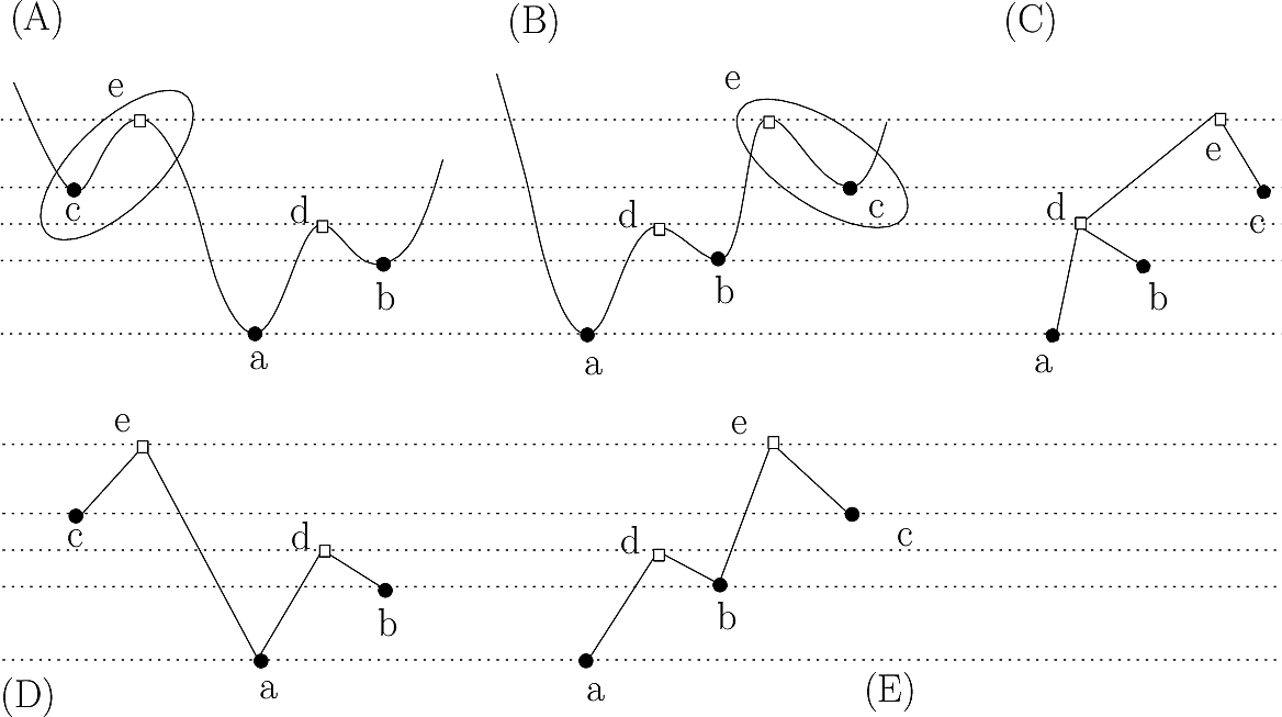
Simplification: strategy using Union-Find versus refined strategy using the Morse-Smale-Witten (MSW) complex. (A,B) Two landscapes, with critical points of indices 0 (disks) and 1 (squares). (C) The disconnectivity graph (DG) of both landscapes, namely the tree depicting the evolution of connected components of sublevel sets. Despite the differences between their MSW complexes, both landscapes share the same DG: upon passing the critical point e, the stable manifold of c merges with that born at a. (D,E) The MSW complexes of (A,B), respectively. In cancelling the pair of critical points (c, e), one does not know from the DG with which (a or b) the basin of c should be merged. But the required information is found in the MSW complex: on the landscape (A), c is merged with a; on the landscape (B), c is merged with b.
Graph connecting sample points versus graph connecting critical points
The Morse based simplification can be applied in two rather different settings:
using a graph connecting points sampling a Morse function,
using a graph connecting critical points only.
In performing the simplification and the re-assignment of points to stable manifold, the question arises to decide whether one should also reassign the stable manifold of saddle points or not.
For example, in simplifying a transition graph representing a molecular energy landscape, one may wish to assign to persistent basins local minima only – but not the saddle points they are connected to, as illustrated on Fig. Fig. fig-pers-tg for an illustration.
Persistence based simplification on a toy landscape with four local minima and four saddle points.
At a persistence threshold p=0.5, only two minima survive, namely the global minimum and . Upon performing the simplification, the minima and flow into , and one is left with a landscape with two basins only: that of whose stable manifold is itself. There are two possibilities for the stable manifolds of these points:
option 1, no re-assignment of SM of saddles: and .
option 2, re-assignment of SM of saddles: and .
Architecture
There are two main packages :
Morse_Smale_Witten_chain_complex : provides the data structure for representing the MSW chain complex, and algorithms to build it from a NNG or a WG.
This section describes the main class to be used in Core algorithms, and the modules to be used in applications.
Main class
The class SBL::GT::T_Morse_theory_based_analyzer has only one template parameter, that is MorseSmaleWittenChainComplex , a representation of the MSW chain complex provided by the package Morse_theory_based_analyzer. Its constructor takes a MSW chain complex and constructs the corresponding disconnectivity forest. It offers the following functionalities.
Critical points and their connections.
The method SBL::GT::T_Morse_theory_based_analyzer::get_paths returns the set of all triples (0-saddle, 1-saddle, 0-saddle) that exists in the underlying MSW chain complex : the saddle points are represented by their vertices in the input MSW chain complex.
This is done so that all points used for building the MSW chain complex are segregated into the stable manifolds of local minima. Note that points associated to saddles of strictly positive index may be arbitrarily assigned to different stable manifolds. To avoid duplication of such points, an arbitrary choice is made, that is, each such point is ascribed to a chosen stable manifold.
Disconnectivity forest.
The disconnectivity forest is the main data structure for understanding how index one saddles are linked together. While processing the saddles of the MSW chain complex by increasing function value, the connected components of points associated to local minima merge. The internal vertices of the disconnectivity forest are exactly the index one saddles from which two different connected components merge.
More precisely, consider the sub-level set of all points that are below a threshold: those points make different components associated to different local minima. When the threshold is under the elevation of the lowest local minimum, the sub-level set is empty. When rising the threshold value, two events may occur :
there is a 0-saddle whose associated value passes under the threshold : a new component is created with the point represented by the 0-saddle, corresponding to a leaf in the disconnectivity forest;
there is a saddle of index one whose associated value passes under the threshold, such that the components of its descendants were not merged : the descendant components are merged into a new one, corresponding to an internal vertex in the disconnectivity forest, linked by edges to the corresponding descendants;
When a point which is not a saddle has an associated value passing under the threshold, it is simply added to the connected component associated to the saddle of this point : there is no change in the disconnectivity forest.
Advanced. The algorithm used for computing the disconnectivity forest is the one described in [89], but applied to vertices of the MSW chain complex. This can be done since all events that occur are associated to the saddles, i.e the vertices of the MSW chain complex.
The persistence of a saddle is the measure of the lifetime of the homological feature associated with this saddle. For example, the persistence of a local minimum is the lifetime of the connected component which gets created at the function value of the minimum.
When two components merge, the smallest component dies while the largest component grows. Hence, the persistence of a saddle s is the difference between the value associated to the saddle where the component of s dies, and the value of s itself. The persistence interval of a saddle is just defined by these two values. When a saddle cannot be merged anymore, it has an infinite persistence.
The persistence diagram is defined as the list of pairs of vertices in the disconnectivity forest such that a component is created at the value of the first vertex, and dies at the value of the second vertex. The list is sorted by ascending values of persistences. Three operations are available on persistence diagrams:
A sub-level set is a component of points as defined previously where all the points are below a given threshold. Hence, all points whose values are below the threshold are assigned to a sub-level set. Assignment refers to the fact that points above the threshold are not included in the sub-level sets, so that sub-level sets are not a partition of all the input points of the MSW chain complex. Accessing the sub-level sets assignment for a given threshold value is done using the method SBL::GT::T_Morse_theory_based_analyzer::get_sublevelsets_connected_components
Simplification.
While all the previous operations aim to access specific analysis on the MSW chain complex, the simplification operation aims to remove the least persistent saddles from the analysis. In particular, it helps to eliminate noise and spurious saddles, so to have more smooth analysis of the MSW chain complex. See Morse_Smale_Witten_chain_complex for a full description of the simplification algorithm. To simplify the MSW chain complex so as to eliminate all saddles having a persistence under a given threshold, one has to use the method SBL::GT::T_Morse_theory_based_analyzer::simplify .
Note that this method simplifies the MSW chain complex and recompute the disconnectivity forest and the persistence diagram.
Morse_theory_based_analyzer_module
Base module.
The module SBL::Modules::T_Morse_theory_based_analyzer_module< ModuleTraits , MorseSmaleWittenChainComplex > is a generic class computing the different described analysis over an input MSW chain. The template parameter MorseSmaleWittenChainComplex is the representation of the MSW chain complex and should be an instantiation of the class SBL::GT::T_Morse_Smale_Witten_chain_complex . When the template parameter ModuleTraits defines the type Morse_Smale_Witten_chain_complex, there is no need of specifying this second template parameter.
In addition to the previously described analysis, the module provides command-line options for customizing the analysis :
–persistence-threshold : removes from the analysis all the saddles with a persistence below the input threshold.
–sublevelset-threshold : computes the sub-level sets by applying the input threshold.
NB: when this option is used, selected samples are filtered out from stable manifolds whose union is computed to define the connected components of sublevel sets. Results are stored in files prefixed with subleveltset_cluster, not to be confused with files prefixed with stable_manifold_cluster (see below).
–keep-largest-ccs : keeps in the displayed disconnectivity forest only the k largest connected components.
–club-saddles : creates into the displayed disconnectivity forest bins of saddles of a given size, representing them as a unique vertex of the forest.
–view-labels : adds into the displayed disconnectivity forest labels for each vertex.
–split-basins : reports each stable manifold of the partition in a separated plain text file, rather than all in the same XML archive file. This feature helps in particular when partitioned points are then used by other programs reading plain text files of points.
NB: when this option is used, stable manifolds, aka clusters, are stored in output files prefixed with stable_manifold_cluster.
When the MSW chain complex has already been computed, it is stored in a XML archive file. It is possible to directly load this XML archive using the option –MSW-filename : this is useful when previous steps for computing the MSW chain complex are time-consuming.
Specialized modules.
Remind that the MSW chain complex can be built from a Nearest Neighbors Graph (NNG), a Weighted Graph (WG), or a Vertex Weighted Graph (VWG). The previous module is specialized for each possible input graph :
SBL::Modules::T_Morse_theory_based_analyzer_for_NNG_module< ModuleTraits > : computes the MSW chain complex from a NNG and performs the described analysis. The template parameter ModuleTraits has to define the types Graph representing the input NNG, Morse_function representing the real-value function over the vertices of the NNG, and Distance_graph_function computing the distance between two vertices of the NNG. An additional command-line option –normalize-gradient allows to normalize the gradient of the associated function by the distances associated to the edges. for analyzing a NNG:
SBL::Modules::T_Morse_theory_based_analyzer_for_weighted_graph_module< ModuleTraits > : computes the MSW chain complex from a WG, and performs the described analysis. When building the MSW chain complex, the edges of the WG are considered as 1-saddles in the MSW chain-complex. The template parameter ModuleTraits has to define the types Graph representing the input WG, and Get_weight computing the weight associated to an edge or a vertex. Note that a WG does not necessarily defines a weight over vertices, so that the class Get_weight has to define this weight.
For example, the weight of a vertex can be the minimum weight over its incident edges, minus a user-defined epsilon value. In all cases, the the value of a vertex is required to be less than the values of its incident edges.
SBL::Modules::T_Morse_theory_based_analyzer_for_vertex_weighted_graph_module< ModuleTraits > : computes the MSW chain complex from a VWG and performs the described analysis. When building the MSW chain complex, the edges of the VWG are considered as 1-saddles in the MSW chain-complex. The template parameter ModuleTraits has to define the types Graph representing the input VWG, and Get_weight computing the weight associated to a vertex of the input VWG.
Note that in using a VWG, weights on edges are not required. If undefined, the maximum weight over the incident vertices is used.
Examples
Using the analyzer
The following example shows how to manually build a MSW chain complex and perform analysis over it. It creates an abstract landscape as a graph where vertices are the critical points of the landscape and edges link neighbors in the landscape. Critical points are actually abstract, meaning that they have no geometrical representation (i.e they are just vertices in a graph). Then, it builds the MSW chain complex by adding the saddles and linking them. Finally, it builds the analyzer engine and displays the different analysis.
This example shows how to use the module SBL::Modules::T_Morse_theory_based_analyzer_for_NNG_module for analyzing an input set of 2D points elevated by input weights. It first computes a NNG of the input set of points, and then computes the MSW chain complex from which the analysis are made.
This example shows how to use the module SBL::Modules::T_Morse_theory_based_analyzer_for_weighted_graph_module for analyzing an input WG, that is an edge weighted graph. Note that the input WG does not define weights over the vertices, but the algorithm requires such weights. Hence, it is the functor Get_weight that defines the weight of a vertex as the minimal weight among its incident edges.
This example shows how to use the module SBL::Modules::T_Morse_theory_based_analyzer_for_vertex_weighted_graph_module for analyzing an input VWG. Note that the input VWG does not define weights over the edges, and the algorithm does not require such weights since they can be estimated from the weights over the vertices.
This package offers also a number of programs applying the analysis to the following cases :
sbl-Morse-theory-based-analyzer-nng-euclid-density-gauss.exe : (i) computes the NNG of a set of points in the Euclidean space, (ii) computes an elevation for each of them based upon a Gaussian based kernel density estimate, (iii) builds the MSW chain complex, and (iv) run the analysis. Note that this construction can in particular be used to perform a density based clustering, with one cluster for each (persistent) mode of the estimated density.
sbl-Morse-theory-based-analyzer-nng-euclid.exe : (i) computes the NNG of a set of elevated points in the Euclidean space, (ii) builds the MSW chain complex with the elevation of the points as function, and (iii) run the analysis.
sbl-Morse-theory-based-analyzer-wg.exe : builds the MSW chain complex associated to the input weighted graph as discussed in the examples, and run the analyis.
sbl-Morse-theory-based-analyzer-vwg.exe : builds the MSW chain complex associated to the input vertex weighted graph as discussed in the examples, and run the analysis.
Main specifications
Below, we list of the specific options of the various executables.
Main options: sbl-Morse-theory-based-analyzer-nng-euclid-density-gauss.exe The main options are:
–points-filestring: The input points in Point_d format –num-neighborsstring: The num of neighbors used to compute the nearest neighbor graph –persistence-thresholdstring: The persistence threshold –split-basinsstring: Report each persistent basin into a separate text file (default is a single serialized xml file)
Main options: sbl-Morse-theory-based-analyzer-nng-euclid-density-gauss.exe
The options are identical to those just described. The only difference is that the elevation is give – as opposed to computed from a density estimation:
–heights-filestring: The elevation of the points – one line per point
Main options: sbl-Morse-theory-based-analyzer-wg.exe
The main options are:
–edges-filestring: The edges of the graph given as pairs of integers -edge-weights-filestring: The weights on the edges
Input. See above.
Main output. The main file generated, common to all programs, are the following ones:
Persistence diagram, txt format, suffix persistence_diagram.txt: point defining the persistence diagram
Persistence diagram, pdf format, suffix persistence_diagram.pdf: plot of the persistence diagram
Disconnectivity forest, eps format, suffix disconnectivity_forest.eps: the forest of binary trees describing merge event between sub/super level-sets.
Cluster leaders, txt file, suffix cluster_leaders.txt: the index of the leading point associated to a basin.
Basins, xml format, suffix stable_manifold_partition.xml: the partition of input samples into basins as selected by the persistence threshold. The first point listed in a basin is its local minimum.
Help on module SBL.sbl_jupyter in SBL:

NAME
    SBL.sbl_jupyter

DESCRIPTION
    ## Load as follows
    #from SBL import sbl_jupyter as sblj
    #help(sblj)
    #
    ## Use as follows
    # sblj.SBLjupyter.find_and_show_images(".png", odir, 50)

CLASSES
    builtins.object
        tools

    class tools(builtins.object)
     |  Static methods defined here:
     |
     |  convert_eps_to_png(ifname, osize)
     |
     |  convert_pdf_to_png(ifname, osize)
     |
     |  find_and_convert(suffix, odir, osize)
     |      # find file with suffix, convert, and return image file
     |
     |  find_and_show_images(suffix, odir, osize)
     |
     |  find_file_in_output_directory(suffix, odir)
     |
     |  show_eps_file(eps_file, osize)
     |
     |  show_image(img)
     |
     |  show_log_file(odir)
     |
     |  show_pdf_file(pdf_file)
     |
     |  show_row_n_images(images, size)
     |
     |  ----------------------------------------------------------------------
     |  Data descriptors defined here:
     |
     |  __dict__
     |      dictionary for instance variables (if defined)
     |
     |  __weakref__
     |      list of weak references to the object (if defined)

FILE
    /user/fcazals/home/projects/proj-soft/sbl/python/SBL/sbl_jupyter.py
Analysing a density estimate with application to density based clustering
As a first illustration, we analyze the density estimated from a point cloud (in 2D here). Using persisstence, we select the most
persistent modes of the estimated density, and retrun one cluster for each mode.
In [2]:
importosimportshutil# python 3 onlyimportmatplotlib.pyplotaspltimportmatplotlib.imageasmplimgfromSBLimportsbl_jupyterassbljdefanalyze_density(ifile,num_neighbors=8,persistence=-1):odir="results-dens"ifos.path.exists(odir):os.system("rm -rf %s"%odir)os.system(("mkdir %s"%odir))exe=shutil.which("sbl-Morse-theory-based-analyzer-nng-euclid-density-gauss.exe")ifexe:cmd="%s --points-file %s --num-neighbors %d --persistence-threshold %.2f\ -d %s"%(exe,ifile,num_neighbors,persistence,odir)print(cmd)os.system(cmd)# find the partition of input points into clusterscmd="find %s -name \"*stable_manifold_partition.xml\""%odirprint(cmd)xml_file=os.popen(cmd).readlines()[0].rstrip()# generate the imagecmd="sbl-clusters-display.py -f %s -c %s -o %s"%(ifile,xml_file,odir)print(cmd)os.system(cmd)# display imagesimages=[]images.append(sblj.tools.find_and_convert("stable_manifold_partition.png",odir,100))images.append(sblj.tools.find_and_convert("disconnectivity_forest.eps",odir,100))images.append(sblj.tools.find_and_convert("persistence_diagram.pdf",odir,100))sblj.tools.show_row_n_images(images,100)else:print("Executable not found")analyze_density("data/points-N200-d50.txt",persistence=-1)analyze_density("data/points-N200-d50.txt",persistence=0.75)
We process a graph with weights on edges. Note that edges of the graph only are required. An edge is a pair of vertices represented by their indices, so that vertices are implicitely created from edge declarations.