|
Structural Bioinformatics Library
Template C++ / Python API for developping structural bioinformatics applications.
|
|
Structural Bioinformatics Library
Template C++ / Python API for developping structural bioinformatics applications.
|
![]()
Authors: S. Bereux and F. Cazals
Multiple Sequence Alignments are pivotal to understand commonalities and differences between protein sequences. Likewise, interface models are pivotal to mine to stability and the specificity of protein interactions. Combining MSA and interface models yields Multiple Interface String Alignment (MISA), namely alignments of strings coding properties of a.a. found at protein-protein interfaces.
Assume the interface of a complex has been found – we do so using the package Space_filling_model_interface . MISA are a visualization tool to display coherently various sequence and structure based statistics for the residues found at this interface, on a chain instance basis. That is, a MISA primarily consists of annotations for chain instances. Currently supported annotations for are:


The benefit of MISA are:
MISA id. A complex 


Likewise, an unbound structure is specified by a sorted list of chain ids 


Our goal is two build one MISA for each so-called MISA id, which we formally define as:


Note that because of th sortedness, a given chain gets the same MISA id in a complex or unbound structure.

Interface strings (i-strings). In the sequel, we present MISA informally. We represent each instance with a so-called interface string encoding properties of amino acids found interfaces involving that chain. The interface string of a chain instance is a character string with one character per residue, and is actually defined from all instances with the same MISA id. To build this character string, we first define:

Using this consensus interface, the residues of a given chain instance (bound or unbound) are displayed as follows:
Finally, assembling i-strings yields MISA:
A colored MISA is a plain MISA whose 1-letter code of a.a. are colored using specific biological / biophysical properties:

A limitation of the BSA is that its calculation uses the geometry of the bound structure only. The calculation is thus oblivious to conformational changes which may be at play in case of induced fit or conformer selection. To mitigate the previous plot, we also provide a the so-called 
Consider an interface partner 


The B-factors reflects the atomic thermal motions. Selected recent crystal structures report this information as a 3x3 ANISOU matrix (the anisotropic B-factor). In order to have a single quantity for all the crystals, the ANISOU matrix 

Optionally, one can choose to normalize the B-factor with respect to (i) all the residues in the chain, or (ii) all the displayed residues.
The package actually provides four complementary scripts:


The reader is referred to section Dependencies and Installation for installation related issues.
In the following, we briefly specify the entry of the scripts provided by this package, and refer the reader to the jupyter notebook of use cases.
This is the main script computing (colored) MISA.
Specification file. The link between Voronoi interfaces and interface strings is done by providing a list of so-called Interface string specifications:
We note that the tag ie string providing extra information is a placeholder to accommodate any relevant information. It should contain only alphanumerical characters, without blank spaces or special characters. For example, the tag may specify a feature (eg open or close) qualifying the crystallized conformation of the chain X.
Such interface string specifications are possibly enriched by specifying windows, ie a list of ranges of amino acids of interest – to be use to restrict the display.
Here is an illustration for the first example provided in the jupyter notebook:
Main options. The main arguments of the script


The script


Specification file. The MISA id and coloring as well as the location of the individual files must be provided. These three pieces of information are provided thanks to a specification file, organized in three lines. Each line begins by a tag which indicates the information type provided on the line :


Here is an illustration for the first example provided in the jupyter notebook:
Main options. Summarizing, here are the main input arguments of the script

The script
Specification file. By default, all residues are processed. A specification file can also be provided to

The specification file then consists of a list of residue identifiers: ![$\text{\texttt{[ residue identifier 1, residue identifier 2...]}}$](form_980_dark.png)
By default, in the absence of such a specification file, the BSA of every residue (with a BSA greater than or equal to 0.01) is displayed.
Here is an illustration for the first example provided in the jupyter notebook:
Main options. The main options are:


The script
Automatic interface specification file. The first consists of extracting it from the 
Here is an illustration for the first example provided in the jupyter notebook, which uses both specifications:
Manual interface specification. The second consists of enumerating the interface in a 

Using this compact residue specification, one can manually specify an interface in an

Here is an illustration for the
Main options. Summarizing, here are the main input arguments of the script
The SBL provides VMD, PyMOL, and Web plugins for sbl-misa.py. Launch the VMD plugin from the SBL catalog under the Extensions menu, start the PyMOL plugin by running sbl_misa in the PyMOL command line, and open the Web plugin from the SBL web plugins launcher page (served locally via sbl-web-plugins-launcher). All three plugins expose the same GUI and capabilities.
 |
| sbl-misa plugin user interface. The user interface for the sbl-misa plugin. The typical workflow is: Step 1: Provide input file. Step 2: Choose an output directory (optional, a default is provided). Step 3: Launch the computation. Step 4: Inspect the interface results in the viewer. Step 5: Review the alignment strings in the GUI. Step 6: (Optional) Use the update panel to select the interface to view in the viewer. |
The analysis provided by the previous scripts involve the following seven steps:
Step 1 : Parsing the input : Parse the specification file and gather the structural data processed
Step 2 : Constructing the MISA: Initializing the MISA by gathering the chains with the same MISA id and aligning them
Step 3 : Coloring the MISA: Collecting the coloring values and attributing the coloring to each chain of the MISA
Step 4 : Recording the cMISA: recording the colored MISA into an HTML file presenting simultaneously the four colorings
Step 5 : Construction of the PDB interface files: storing the interface residues shared by each pair of chain into PDB files
Step 6 : Computation of the i-RMSD for each pair of chain: computing the iRMSD for each pair of PDB interface files
Step 7 : Analysis of the interface RMSD (i-RMSD): clustering the chains according to the iRMSD and recording statistics on the iRMSD
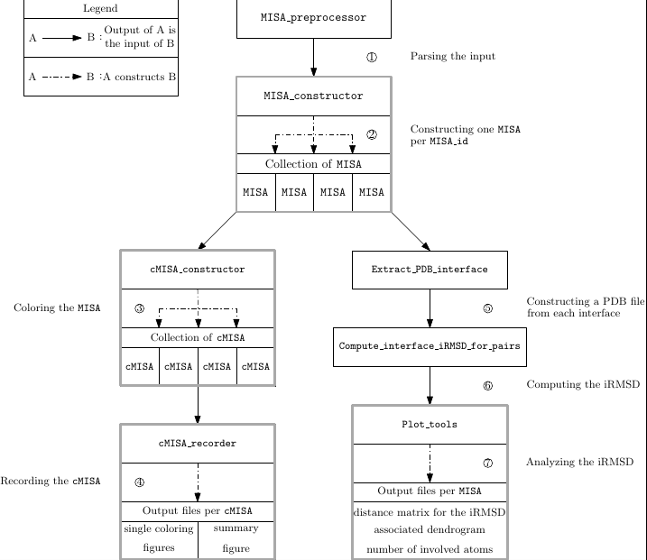 |
| Overview of sbl-misa.py |
Dictionary of Secondary Structures (DSSP). DSSP [115] : DSSP . The package DSSP is used to infer the type of secondary structure element a given aa belong to. The program mkdssp used is described here; one may also consult directly the source code. executable: 
DSSP is provided by package managers. For example, it is easily installed as follows under Fedora
dnf install dssp.x86_64
Multi Sequence Alignment. We compute Multi Sequence Alignment with ClustalOmega [180] To install ClustalOmega, proceed as indicated on the web site ClustalOmega .
Python packages. The following python packages are used:
All of them are easily installed as follows:
pip3 install biopython numpy scipy pandas matplotlib weasyprint seaborn
We first list the required packages from the SBL, and then detail the two options supported to install these packages.
List of SBL packages. The computation of MISAs uses the following packages from the SBL:


Installation using package managers. One can install the executables and python scripts available within packages using package managers , (dnf or rpm under Linux Fedora). In short:
> dnf install sbl-VERSIONNUMBER-Linux-apps.rpm
> dnf install sbl-VERSIONNUMBER-Linux-scripts.rpm
Installation upon git cloning the SBL. As explained in the installation guide, one can git clone the SBL, and compile the whole library, or more specifically the packages required, namely Space_filling_model_interface, Buried_surface_area and Space_filling_model_surface_volume.
To clone the SBL, proceed as indicated here. To compile the SBL or the required packages, follow the Compilation and installation .
Remark. Whatever the installation method used, make sure all executables and python scripts are visible from one's PATH environment variable.
See the following jupyter notebook:
The following notebook uses a number of files provided in the following directories: ```pdb misa-RBD-ACE2-cmp misa-RBD-IG'''
This first example provides a step by step comparison on the RBD.
First, the MISA is calculated for each of the chains specified in ifile-misa.txt.
Content of ./misa-RBD-ACE2-cmp/ifile-misa.txt :
# Windows for ACE2-bound-to-SARS-CoV-1
[ACE2-bound-to-SARS-CoV-1_0 (19, 83) (321,393)]

./pdb/2ajf.pdb (A, E, SARS-CoV-1-RBD, bound) (B, A, ACE2-bound-to-SARS-CoV-1, bound)
./pdb/2ajf.pdb (A, F, SARS-CoV-1-RBD, bound) (B, B, ACE2-bound-to-SARS-CoV-1, bound)
./pdb/5x58.pdb (A, A, SARS-CoV-1-RBD, unbound-closed)
./pdb/6crz.pdb (A, C, SARS-CoV-1-RBD, unbound-closed)

# Specification for SARS-CoV-2
./pdb/6m0j.pdb (C, E, SARS-CoV-2-RBD, bound) (D, A, ACE2-bound-to-SARS-CoV-2, bound)
./pdb/6lzg.pdb (C, B, SARS-CoV-2-RBD, bound) (D, A, ACE2-bound-to-SARS-CoV-2, bound)
./pdb/6vxx.pdb (C, A, SARS-CoV-2-RBD, unbound-closed)
./pdb/6vyb.pdb (C, A, SARS-CoV-2-RBD, unbound-closed)
Each line corresponds to a complex, or to an unbound structure if the structure is alone on its line. For each complex, we provided one or two examples of bound complexes, as well as two examples of unbound complexes, in order to be able to calculate the $\Delta\_ASA$ induced by the conformational change. Otherwise, the $\Delta\_ASA$ won't be computed.
The first line of the file is used to restrict the displayed portion of the interface for the SARS-CoV-1 RBD, in order to compact the output.
The details of the specification are developed in the paper.
#!/usr/bin/python3
import os
import subprocess
import re
import shutil
from IPython.core.display import display, HTML
from collections import defaultdict
from IPython.display import IFrame
from SBL import SBL_pytools
from SBL_pytools import SBL_pytools as sblpyt
exe        = shutil.which('sbl-misa.py')
if not exe: # if exe == None
    print('sbl-misa.py not in your PATH')
ifile              = './misa-RBD-ACE2-cmp/ifile-misa.txt'
prefix_dir         = './misa-RBD-ACE2-cmp' # To append at the beginning of every input and output directories
# It allows to compacify the possible specification of the sub-output directories.

prefix             = 'demo-misa-1' # To append at the beginning of the output files
verbose            = '0'
normalize_b_factor = '2' # Normalization with only respect to the displayed residues
cmd                = [exe, "-ifile", ifile, "-prefix_dir", prefix_dir, '-prefix', prefix, '--verbose', verbose, '-normalize_b_factor', normalize_b_factor]
print('Running %s -ifile %s -prefix_dir %s -prefix %s --verbose %s -normalize_b_factor %s' % (exe, ifile, prefix_dir, prefix, verbose, normalize_b_factor))
s                  = subprocess.check_output(cmd, encoding='UTF-8')
print('\nDone')
#print(s)
Running /user/fcazals/home/projects/proj-soft/sbl-install/lib/python3.8/site-packages/SBL/sbl-misa.py -ifile ./misa-RBD-ACE2-cmp/ifile-misa.txt -prefix_dir ./misa-RBD-ACE2-cmp -prefix demo-misa-1 --verbose 0 -normalize_b_factor 2

Done
sbl-misa.py displays the MISA, with several colorings showing complementary data.
An individual summary figure for each of the chains specified in ifile-misa.txt is produced. For example, here are the figures generated for SARS-CoV-2-RBD and for SARS-CoV-1-ACE2 (for which the effect of the window specification, restricting the range of displayed residues, can be observed) :
#IFrame(src='./misa-RBD-ACE2-cmp/MISA/SARS-CoV-2-RBD_0-demo-misa-1.html', width="100%", height=600)
display(HTML('./misa-RBD-ACE2-cmp/MISA/SARS-CoV-2-RBD_0-demo-misa-1.html'))
Legend for the amino acids (aa) encoding : For aa not at the interface : _ if aa is missing - if aa is present For aa at the interface : * if aa is missing X if consensus aa (= most frequent among the bound structures, and in case of tie the first by alphabetical order) x otherwise (For bound structure files only) : x or X if the aa is part of the consensus interface but not part of the interface of this fileMISA SSE for MISA-ID SARS-CoV-2-RBD_03-turn helix - 4-turn helix - 5-turn helix - Isolated beta-bridge residue - Extended strand - Bend - Hydrogen bonded turn - Other - Missing Residue - Residue Index 403----410-------420-------430-------440-------450-------460-------470-------480-------490-------500---- | | | | | | | | | | | bound-6m0j-E, res :2.45 Å, 27 interf res R-DE----------KI--Y-----------------N-----VGG-Y---Y-LF----------------Y-AGS------EGFN-YF-LQSYGFQPTNGVGYQ bound-6lzg-B, res :2.5 Å, 39 interf res R-DE----------KI--Y-----------------N-----VGG-Y---Y-LF----------------Y-AGS------EGFN-YF-LQSYGFQPTNGVGYQ unbound-closed-6vxx-A, res :2.8 Å, 0 interf res R-DE----------KI--Y-----------------N-----**G-Y---Y-**_____-------____*_***______****_YF-LQSYGFQPTN*VGYQ unbound-closed-6vyb-A, res :3.2 Å, 0 interf res R-DE----------KI--Y-----------------N---__***-Y---Y-LF--------------__*_***______****_*F-LQSYGFQPTN*VGYQMISA BSA for MISA-ID SARS-CoV-2-RBD_0In dark grey, residues with missing data for coloring Buried Surface Area (BSA) (in Å2)| bound-6m0j-E : total bsa = 887.29 Å2 | bound-6lzg-B : total bsa = 1120.20 Å2 Residue Index 403----410-------420-------430-------440-------450-------460-------470-------480-------490-------500---- | | | | | | | | | | | bound-6m0j-E, res :2.45 Å, 27 interf res R-DE----------KI--Y-----------------N-----VGG-Y---Y-LF----------------Y-AGS------EGFN-YF-LQSYGFQPTNGVGYQ bound-6lzg-B, res :2.5 Å, 39 interf res R-DE----------KI--Y-----------------N-----VGG-Y---Y-LF----------------Y-AGS------EGFN-YF-LQSYGFQPTNGVGYQ
MISA Delta_ASA for MISA-ID SARS-CoV-2-RBD_0In dark grey, residues with missing data for coloring Bound structures : In light grey residues in bound structure for which miss corresponding ASA values in the unbound structures Per residue i, delta_ASA = ASA[i] - mean(ASA[i]) (mean is computed using the unbound structures) (in Å2)Unbound structures : Accessible Surface Area (ASA) (in Å2)
Residue Index 403----410-------420-------430-------440-------450-------460-------470-------480-------490-------500---- | | | | | | | | | | | bound-6m0j-E, res :2.45 Å, 27 interf res R-DE----------KI--Y-----------------N-----VGG-Y---Y-LF----------------Y-AGS------EGFN-YF-LQSYGFQPTNGVGYQ bound-6lzg-B, res :2.5 Å, 39 interf res R-DE----------KI--Y-----------------N-----VGG-Y---Y-LF----------------Y-AGS------EGFN-YF-LQSYGFQPTNGVGYQ unbound-closed-6vxx-A, res :2.8 Å, 0 interf res R-DE----------KI--Y-----------------N-----**G-Y---Y-**_____-------____*_***______****_YF-LQSYGFQPTN*VGYQ unbound-closed-6vyb-A, res :3.2 Å, 0 interf res R-DE----------KI--Y-----------------N---__***-Y---Y-LF--------------__*_***______****_*F-LQSYGFQPTN*VGYQ
MISA B_factor for MISA-ID SARS-CoV-2-RBD_0In dark grey, residues with missing data for coloring B-Factor (in Å2)Residue Index 403----410-------420-------430-------440-------450-------460-------470-------480-------490-------500---- | | | | | | | | | | | bound-6m0j-E, res :2.45 Å, 27 interf res R-DE----------KI--Y-----------------N-----VGG-Y---Y-LF----------------Y-AGS------EGFN-YF-LQSYGFQPTNGVGYQ bound-6lzg-B, res :2.5 Å, 39 interf res R-DE----------KI--Y-----------------N-----VGG-Y---Y-LF----------------Y-AGS------EGFN-YF-LQSYGFQPTNGVGYQ unbound-closed-6vxx-A, res :2.8 Å, 0 interf res R-DE----------KI--Y-----------------N-----**G-Y---Y-**_____-------____*_***______****_YF-LQSYGFQPTN*VGYQ unbound-closed-6vyb-A, res :3.2 Å, 0 interf res R-DE----------KI--Y-----------------N---__***-Y---Y-LF--------------__*_***______****_*F-LQSYGFQPTN*VGYQ
#IFrame(src='./misa-RBD-ACE2-cmp/MISA/ACE2-bound-to-SARS-CoV-1_0-demo-misa-1.html', width="100%", height=600)
display(HTML('misa-RBD-ACE2-cmp/MISA/ACE2-bound-to-SARS-CoV-1_0-demo-misa-1.html'))
Legend for the amino acids (aa) encoding : For aa not at the interface : _ if aa is missing - if aa is present For aa at the interface : * if aa is missing X if consensus aa (= most frequent among the bound structures, and in case of tie the first by alphabetical order) x otherwise (For bound structure files only) : x or X if the aa is part of the consensus interface but not part of the interface of this fileMISA SSE for MISA-ID ACE2-bound-to-SARS-CoV-1_03-turn helix - 4-turn helix - 5-turn helix - Isolated beta-bridge residue - Extended strand - Bend - Hydrogen bonded turn - Other - Missing Residue - Residue Index -20--------30--------40--------50--------60--------70--------80-- 321------330-------340-------350-------360-------370-------380-------390- | | | | | | | | | | | | | | | bound-2ajf-A, res :2.9 Å, 33 interf res S---EQ-KTF-DK--H--ED--YQ--L---------------------------------L--MY ---TQGF-EN----------------------KGDFR----------------------------AAQP---R bound-2ajf-B, res :2.9 Å, 27 interf res S---EQ-KTF-DK--H--ED--YQ--L---------------------------------L--MY ---TQGF-EN----------------------KGDFR----------------------------AAQP---RMISA BSA for MISA-ID ACE2-bound-to-SARS-CoV-1_0In dark grey, residues with missing data for coloring Buried Surface Area (BSA) (in Å2)| bound-2ajf-A : total bsa = 888.38 Å2 | bound-2ajf-B : total bsa = 817.21 Å2 Residue Index -20--------30--------40--------50--------60--------70--------80-- 321------330-------340-------350-------360-------370-------380-------390- | | | | | | | | | | | | | | | bound-2ajf-A, res :2.9 Å, 33 interf res S---EQ-KTF-DK--H--ED--YQ--L---------------------------------L--MY ---TQGF-EN----------------------KGDFR----------------------------AAQP---R bound-2ajf-B, res :2.9 Å, 27 interf res S---EQ-KTF-DK--H--ED--YQ--L---------------------------------L--MY ---TQGF-EN----------------------KGDFR----------------------------AAQP---R
MISA Delta_ASA for MISA-ID ACE2-bound-to-SARS-CoV-1_0In dark grey, residues with missing data for coloring Bound structures : In light grey residues in bound structure for which miss corresponding ASA values in the unbound structures Per residue i, delta_ASA = ASA[i] - mean(ASA[i]) (mean is computed using the unbound structures) (in Å2)Unbound structures : Accessible Surface Area (ASA) (in Å2)
Residue Index -20--------30--------40--------50--------60--------70--------80-- 321------330-------340-------350-------360-------370-------380-------390- | | | | | | | | | | | | | | | bound-2ajf-A, res :2.9 Å, 33 interf res S---EQ-KTF-DK--H--ED--YQ--L---------------------------------L--MY ---TQGF-EN----------------------KGDFR----------------------------AAQP---R bound-2ajf-B, res :2.9 Å, 27 interf res S---EQ-KTF-DK--H--ED--YQ--L---------------------------------L--MY ---TQGF-EN----------------------KGDFR----------------------------AAQP---R
MISA B_factor for MISA-ID ACE2-bound-to-SARS-CoV-1_0In dark grey, residues with missing data for coloring B-Factor (in Å2)Residue Index -20--------30--------40--------50--------60--------70--------80-- 321------330-------340-------350-------360-------370-------380-------390- | | | | | | | | | | | | | | | bound-2ajf-A, res :2.9 Å, 33 interf res S---EQ-KTF-DK--H--ED--YQ--L---------------------------------L--MY ---TQGF-EN----------------------KGDFR----------------------------AAQP---R bound-2ajf-B, res :2.9 Å, 27 interf res S---EQ-KTF-DK--H--ED--YQ--L---------------------------------L--MY ---TQGF-EN----------------------KGDFR----------------------------AAQP---R
Once these individual figures have been generated, a call to sbl-misa-mix.py allows to simultaneously compare different MISA_id in the same figure. In the sequel, we focus on the following three colored MISA: SSE, BSA, Delta_ASA,
sbl-misa-mix.py parses the specification file ifile-misa-mix.txt, from which it finds the location of the directory containing the input data, the MISA_id to be displayed, and the colorings to be displayed.
Content of ./misa-RBD-ACE2-cmp/ifile-misa-mix.txt :
# List of input directories
localisation (./misa-RBD-ACE2-cmp/MISA)

# List of MISA_chain_ids
misa_chain_id (SARS-CoV-1-RBD_0, SARS-CoV-2-RBD_0)

# List of colorings of interest
coloring (SSE, BSA, Delta_ASA)exe = shutil.which('sbl-misa-mix.py')
if not exe: # if exe == None
print('sbl-misa-mix.py not in your PATH')
prefix = 'demo-mix-1' # To append at the beginning of the output files
mix_ifile = './misa-RBD-ACE2-cmp/ifile-misa-mix.txt' # Specification file
odir = './misa-RBD-ACE2-cmp' # Output directory
verbose = '0'
cmd = [exe, "-mix_ifile", mix_ifile, '-prefix', prefix, '-odir', odir, '--verbose', verbose]
print('Running %s -mix_ifile %s -prefix %s -odir %s --verbose %s' % (exe, mix_ifile, prefix, odir, verbose))
s = subprocess.check_output(cmd, encoding='UTF-8')
print('\nDone')
#print(s)
Running /user/fcazals/home/projects/proj-soft/sbl-install/lib/python3.8/site-packages/SBL/sbl-misa-mix.py -mix_ifile ./misa-RBD-ACE2-cmp/ifile-misa-mix.txt -prefix demo-mix-1 -odir ./misa-RBD-ACE2-cmp --verbose 0

Done
The first figure of the article corresponds to the output of sbl-misa-mix.py , run with the ifile-misa-mix.txt presented above :
#IFrame(src='./misa-RBD-ACE2-cmp/demo-mix-1_SSE_BSA_Delta_ASA_SARS-CoV-1-RBD_0_SARS-CoV-2-RBD_0_mixed_figure.html', width="100%", height=600)
display(HTML('./misa-RBD-ACE2-cmp/demo-mix-1_SSE_BSA_Delta_ASA_SARS-CoV-1-RBD_0_SARS-CoV-2-RBD_0_mixed_figure.html'))
Legend for the amino acids (aa) encoding : For aa not at the interface : _ if aa is missing - if aa is present For aa at the interface : * if aa is missing X if consensus aa (= most frequent among the bound structures, and in case of tie the first by alphabetical order) x otherwise (For bound structure files only) : x or X if the aa is part of the consensus interface but not part of the interface of this file )MISA SSE for MISA-ID SARS-CoV-1-RBD_03-turn helix - 4-turn helix - 5-turn helix - Isolated beta-bridge residue - Extended strand - Bend - Hydrogen bonded turn - Other - Missing Residue - Residue Index 390-------400-------410-------420-------430-------440-------450-------460-------470-------480-------490 | | | | | | | | | | | bound-2ajf-E, res :2.9 Å, 29 interf res K--D--Q-------VI--Y-----------------R-----S---Y---Y-YL----------------F-PD------P-LNCY---NDYG-YTTTGI-YQ bound-2ajf-F, res :2.9 Å, 29 interf res K--D--Q-------VI--Y-----------------R-----S---Y---Y-YL----------------F-PD------P-LNCY---NDYG-YTTTGI-YQ unbound-closed-5x58-A, res :3.2 Å, 0 interf res K--D--Q-------VI--Y-----------------R-----S---Y---Y-YL----------------F-PD------P-LNCY---NDYG-YTTTGI-YQ unbound-closed-6crz-C, res :3.3 Å, 0 interf res K--D--Q-------VI--Y-----------------R-----S---Y---Y-YL----------------F-PD------P-LNCY---NDYG-YTTTGI-YQMISA SSE for MISA-ID SARS-CoV-2-RBD_03-turn helix - 4-turn helix - 5-turn helix - Isolated beta-bridge residue - Extended strand - Bend - Hydrogen bonded turn - Other - Missing Residue - Residue Index 403----410-------420-------430-------440-------450-------460-------470-------480-------490-------500---- | | | | | | | | | | | bound-6m0j-E, res :2.45 Å, 27 interf res R-DE----------KI--Y-----------------N-----VGG-Y---Y-LF----------------Y-AGS------EGFN-YF-LQSYGFQPTNGVGYQ bound-6lzg-B, res :2.5 Å, 39 interf res R-DE----------KI--Y-----------------N-----VGG-Y---Y-LF----------------Y-AGS------EGFN-YF-LQSYGFQPTNGVGYQ unbound-closed-6vxx-A, res :2.8 Å, 0 interf res R-DE----------KI--Y-----------------N-----**G-Y---Y-**_____-------____*_***______****_YF-LQSYGFQPTN*VGYQ unbound-closed-6vyb-A, res :3.2 Å, 0 interf res R-DE----------KI--Y-----------------N---__***-Y---Y-LF--------------__*_***______****_*F-LQSYGFQPTN*VGYQMISA BSA for MISA-ID SARS-CoV-1-RBD_0In dark grey, residues with missing data for coloring Buried Surface Area (BSA) (in Å2)| bound-2ajf-E : total bsa = 925.41 Å2 | bound-2ajf-F : total bsa = 864.87 Å2 Residue Index 390-------400-------410-------420-------430-------440-------450-------460-------470-------480-------490 | | | | | | | | | | | bound-2ajf-E, res :2.9 Å, 29 interf res K--D--Q-------VI--Y-----------------R-----S---Y---Y-YL----------------F-PD------P-LNCY---NDYG-YTTTGI-YQ bound-2ajf-F, res :2.9 Å, 29 interf res K--D--Q-------VI--Y-----------------R-----S---Y---Y-YL----------------F-PD------P-LNCY---NDYG-YTTTGI-YQ
MISA BSA for MISA-ID SARS-CoV-2-RBD_0In dark grey, residues with missing data for coloring Buried Surface Area (BSA) (in Å2)MISA Delta_ASA for MISA-ID SARS-CoV-1-RBD_0In dark grey, residues with missing data for coloring Bound structures : In light grey residues in bound structure for which miss corresponding ASA values in the unbound structures Per residue i, delta_ASA = ASA[i] - mean(ASA[i]) (mean is computed using the unbound structures) (in Å2)Unbound structures : Accessible Surface Area (ASA) (in Å2)
Residue Index 390-------400-------410-------420-------430-------440-------450-------460-------470-------480-------490 | | | | | | | | | | | bound-2ajf-E, res :2.9 Å, 29 interf res K--D--Q-------VI--Y-----------------R-----S---Y---Y-YL----------------F-PD------P-LNCY---NDYG-YTTTGI-YQ bound-2ajf-F, res :2.9 Å, 29 interf res K--D--Q-------VI--Y-----------------R-----S---Y---Y-YL----------------F-PD------P-LNCY---NDYG-YTTTGI-YQ unbound-closed-5x58-A, res :3.2 Å, 0 interf res K--D--Q-------VI--Y-----------------R-----S---Y---Y-YL----------------F-PD------P-LNCY---NDYG-YTTTGI-YQ unbound-closed-6crz-C, res :3.3 Å, 0 interf res K--D--Q-------VI--Y-----------------R-----S---Y---Y-YL----------------F-PD------P-LNCY---NDYG-YTTTGI-YQ
MISA Delta_ASA for MISA-ID SARS-CoV-2-RBD_0In dark grey, residues with missing data for coloring Bound structures : In light grey residues in bound structure for which miss corresponding ASA values in the unbound structures Per residue i, delta_ASA = ASA[i] - mean(ASA[i]) (mean is computed using the unbound structures) (in Å2)
To further the study of an interface, we recover the BSA value of specific user defined residues. This is the purpose of sbl-misa-bsa.py .
We provide to the program an .xml file generated by sbl-intervor-ABW-atomic.exe (run with the --output-prefix option), as well as a specfile containing the list of residues of interest, as presented below :
Content of ./misa-RBD-ACE2-cmp/ifile-misa-bsa.txt :
[(A, E, 303), (A, E, 403), (A, E, 449), (A, E, 455), (A, E, 486), (A, E, 502), (B, A, 79), (B, A, 35)]
exe      = shutil.which('sbl-misa-bsa.py')
if not exe: # if exe == None
    print('sbl-misa-bsa.py not in your PATH')
specfile = './misa-RBD-ACE2-cmp/ifile-misa-bsa.txt' # Path to the spec file containing the list of resid to be studied
xmlfile  = './misa-RBD-ACE2-cmp/input-data/intervor/sbl-intervor-ABW-atomic__radius_water_1dot4__f_6m0j__p_4__P_E__P_A___alpha_0__buried_surface_area.xml' # Name of the .xml input file
cmd       = [exe, "-specfile", specfile, '-xmlfile', xmlfile]
s         = subprocess.check_output(cmd, encoding='UTF-8')
print(s)
Running sbl-misa-bsa.py
XML: 1 / 1 files were loaded

####################################################
BSA for the intervor_partner A

First according to the provided list of residues :

Chain E Residue 303 : bsa = NA Å^2
Chain E Residue 486 : bsa = 98.531 Å^2
Chain E Residue 502 : bsa = 41.882 Å^2
Chain E Residue 455 : bsa = 41.547 Å^2
Chain E Residue 449 : bsa = 37.186 Å^2
Chain E Residue 403 : bsa = 0.096 Å^2

Cumulated bsa for intervor_partner A - chain E is 219.242 Å^2
Cumulated bsa for intervor_partner A is 219.242 Å^2

Then for the other residues (we only display the residues with a BSA greater than 0.001 Å^2) :

Chain E Residue 500 : bsa = 91.397 Å^2
Chain E Residue 505 : bsa = 86.628 Å^2
Chain E Residue 489 : bsa = 73.470 Å^2
Chain E Residue 493 : bsa = 60.387 Å^2
Chain E Residue 498 : bsa = 55.658 Å^2
Chain E Residue 456 : bsa = 45.129 Å^2
Chain E Residue 475 : bsa = 38.708 Å^2
Chain E Residue 487 : bsa = 38.399 Å^2
Chain E Residue 501 : bsa = 30.063 Å^2
Chain E Residue 417 : bsa = 27.641 Å^2
Chain E Residue 496 : bsa = 22.986 Å^2
Chain E Residue 453 : bsa = 22.979 Å^2
Chain E Residue 503 : bsa = 21.688 Å^2
Chain E Residue 484 : bsa = 13.355 Å^2
Chain E Residue 446 : bsa = 10.431 Å^2
Chain E Residue 476 : bsa = 10.198 Å^2
Chain E Residue 445 : bsa = 9.552 Å^2
Chain E Residue 473 : bsa = 6.310 Å^2
Chain E Residue 490 : bsa = 1.404 Å^2
Chain E Residue 477 : bsa = 1.387 Å^2
Chain E Residue 485 : bsa = 0.278 Å^2

Cumulated bsa for intervor_partner A - chain E is 668.049 Å^2
Cumulated bsa for intervor_partner A is 668.049 Å^2


The bsa for intervor_partner A is 668.049 Å^2 (with respect to the provided residue ids)

####################################################
BSA for the intervor_partner B

First according to the provided list of residues :

Chain A Residue 79 : bsa = 24.518 Å^2
Chain A Residue 35 : bsa = 17.735 Å^2

Cumulated bsa for intervor_partner B - chain A is 42.254 Å^2
Cumulated bsa for intervor_partner B is 42.254 Å^2

Then for the other residues (we only display the residues with a BSA greater than 0.001 Å^2) :

Chain A Residue 353 : bsa = 97.689 Å^2
Chain A Residue 31 : bsa = 93.757 Å^2
Chain A Residue 34 : bsa = 68.567 Å^2
Chain A Residue 27 : bsa = 66.460 Å^2
Chain A Residue 24 : bsa = 53.133 Å^2
Chain A Residue 42 : bsa = 44.506 Å^2
Chain A Residue 41 : bsa = 43.731 Å^2
Chain A Residue 30 : bsa = 40.852 Å^2
Chain A Residue 83 : bsa = 38.720 Å^2
Chain A Residue 38 : bsa = 34.191 Å^2
Chain A Residue 354 : bsa = 31.103 Å^2
Chain A Residue 330 : bsa = 28.685 Å^2
Chain A Residue 82 : bsa = 28.595 Å^2
Chain A Residue 45 : bsa = 25.525 Å^2
Chain A Residue 324 : bsa = 17.235 Å^2
Chain A Residue 28 : bsa = 16.649 Å^2
Chain A Residue 37 : bsa = 16.266 Å^2
Chain A Residue 355 : bsa = 11.668 Å^2
Chain A Residue 357 : bsa = 11.206 Å^2
Chain A Residue 19 : bsa = 10.478 Å^2
Chain A Residue 393 : bsa = 9.348 Å^2
Chain A Residue 325 : bsa = 8.452 Å^2
Chain A Residue 326 : bsa = 4.140 Å^2
Chain A Residue 386 : bsa = 0.593 Å^2

Cumulated bsa for intervor_partner B - chain A is 801.550 Å^2
Cumulated bsa for intervor_partner B is 801.550 Å^2


The bsa for intervor_partner B is 801.550 Å^2 (with respect to the provided residue ids)


Done
sbl-misa-diff.py allows to compare the interface between two peer chains, identifying the residues specific to each, and the shared residues, as well as displaying the BSA of these residues.
It allows to compare Voronoi interfaces and/or manually defined interfaces.
Hand-defined interfaces shall be specified in the same format as SARS-CoV-1-RBD-Harisson-2005.txt (see below), where the first line corresponds to the name given to the chain, and each subsequent line corresponds to a residue (nature + index).
Content of ./misa-RBD-ACE2-cmp/SARS-CoV-1-RBD-Harisson-2005.txt :
harisson-interface
T402
R426
Y436
Y440
Y442
L472
N473
Y475
N479
Y484
T486
T487
G488
Y491
The corresponding specfile is the following :
Content of ./misa-RBD-ACE2-cmp/ifile-misa-diff.txt :
(./misa-RBD-ACE2-cmp/MISA/raw-data, 2ajf, E)
(./misa-RBD-ACE2-cmp/SARS-CoV-1-RBD-Harisson-2005.txt)
The output .txt file is displayed below.
exe      = shutil.which('sbl-misa-diff.py')
if not exe: # if exe == None
    print('sbl-misa-diff.py not in your PATH')
specfile = './misa-RBD-ACE2-cmp/ifile-misa-diff.txt'
odir     = './misa-RBD-ACE2-cmp' # Outp
cmd = [exe, "-specfile", specfile, "-odir", odir]
s = subprocess.check_output(cmd, encoding='UTF-8')
print(s)
#sblpyt.show_this_text_file('misa-RBD-ACE2-cmp/comparison-interface-2ajf-E-with-Harisson-interface-RBD-CoV1-ACE2-Science-2005.txt')
sblpyt.show_this_text_file('misa-RBD-ACE2-cmp/comparison-interface-2ajf-E-with-harisson-interface.txt')
Running sbl-misa-diff.py
Reading spec file
Reading interface file
Comparing interfaces
created ./misa-RBD-ACE2-cmp/comparison-interface-2ajf-E-with-harisson-interface.txt
Done


++Showing file misa-RBD-ACE2-cmp/comparison-interface-2ajf-E-with-harisson-interface.txt
Comparison of the Buried Surface Area (BSA) and of the nature of the residues for the interface residues.
(Missing data are denoted by "NA")

16 exclusive residues at the interface of chain 2ajf-E :
            BSA-2ajf-E Names-2ajf-E
( , 390,  )       9.34            K
( , 393,  )       4.92            D
( , 404,  )      14.90            V
( , 405,  )       1.66            I
( , 408,  )       3.25            Y
( , 432,  )       6.46            S
( , 443,  )      34.93            L
( , 460,  )       3.21            F
( , 462,  )      49.79            P
( , 463,  )      11.89            D
( , 470,  )       2.18            P
( , 480,  )       0.45            D
( , 481,  )      11.17            Y
( , 482,  )      14.59            G
( , 489,  )      32.87            I
( , 492,  )       3.55            Q

1 exclusive residues at the interface of chain harisson-interface :
            BSA-harisson-interface Names-harisson-interface
( , 402,  )                     NA                       NA

13 shared residues :
            BSA-2ajf-E BSA-harisson-interface Names-2ajf-E Names-harisson-interface
( , 426,  )      42.57                     NA            R                       NA
( , 436,  )      36.67                     NA            Y                       NA
( , 440,  )      32.86                     NA            Y                       NA
( , 442,  )      60.05                     NA            Y                       NA
( , 472,  )      75.32                     NA            L                       NA
( , 473,  )      51.06                     NA            N                       NA
( , 475,  )      83.14                     NA            Y                       NA
( , 479,  )      23.05                     NA            N                       NA
( , 484,  )      62.65                     NA            Y                       NA
( , 486,  )      86.47                     NA            T                       NA
( , 487,  )      43.74                     NA            T                       NA
( , 488,  )      41.77                     NA            G                       NA
( , 491,  )      80.91                     NA            Y                       NA
--Done
This figure compares the RBD interface of SARS-CoV-1 and SARS-CoV-2 with ACE2, or with different immunoglobulins (VHH72, CR3022, 2F6).
The RBD from SARS-CoV-2 is implied in several complexes, but a same structure cannot simultaneously appears more than once. It is thus necessary to make one ifile-misa.txt per complex. One subdirectory per complex, containing only the relevant ifile-misa.txt was provided.
Each ifile-misa.txt contains one or two examples of bound RBD, as well as two examples of unbound RBD, in order to be able to calculate the $\delta_{ASA}$ induced by the conformational change.
Content of ./misa-RBD-IG/RBD-VHH72/ifile-misa.txt :
./pdb/6waq.pdb (A, B, SARS-CoV-1-RBD-bound-to-VHH72, bound) (B, A, VHH72, bound)
./pdb/5x58.pdb (A, A, SARS-CoV-1-RBD-bound-to-VHH72, unbound-closed)
./pdb/6crz.pdb (A, C, SARS-CoV-1-RBD-bound-to-VHH72, unbound-closed)
Content of ./misa-RBD-IG/RBD-ACE2/ifile-misa.txt :
[SARS-CoV-2-RBD-bound-to-ACE2_0 (346, 528)]
[SARS-CoV-2-RBD-bound-to-ACE2_0 (355, 494)]

# Specification SARS-CoV-1
./pdb/2ajf.pdb (A, E, SARS-CoV-1-RBD-bound-to-ACE2, bound) (B, A, ACE2-bound-to-CoV-1, bound)
./pdb/2ajf.pdb (A, F, SARS-CoV-1-RBD-bound-to-ACE2, bound) (B, B, ACE2-bound-to-CoV-1, bound)
./pdb/5x58.pdb (A, A, SARS-CoV-1-RBD-bound-to-ACE2, unbound-closed)
./pdb/6crz.pdb (A, C, SARS-CoV-1-RBD-bound-to-ACE2, unbound-closed)

# Specification SARS-CoV-2
./pdb/6m0j.pdb (A, E, SARS-CoV-2-RBD-bound-to-ACE2, bound) (B, A, ACE2-bound-to-CoV-2, bound)
./pdb/6lzg.pdb (A, B, SARS-CoV-2-RBD-bound-to-ACE2, bound) (B, A, ACE2-bound-to-CoV-2, bound)
./pdb/6vxx.pdb (A, A, SARS-CoV-2-RBD-bound-to-ACE2, unbound-closed)
./pdb/6vyb.pdb (A, A, SARS-CoV-2-RBD-bound-to-ACE2, unbound-closed)
Content of ./misa-RBD-IG/RBD-CR3022/ifile-misa.txt
[SARS-CoV-2-RBD-bound-to-CR3022_0 (346, 528)]
./pdb/6yla.pdb (A, E, SARS-CoV-2-RBD-bound-to-CR3022, bound) (B, H, CR3022-antibody, bound) (B, L, CR3022-antibody, bound)
./pdb/6yla.pdb (A, A, SARS-CoV-2-RBD-bound-to-CR3022, bound) (B, B, CR3022-antibody, bound) (B, C, CR3022-antibody, bound)
./pdb/6vxx.pdb (A, A, SARS-CoV-2-RBD-bound-to-CR3022, unbound-closed)
./pdb/6vyb.pdb (A, A, SARS-CoV-2-RBD-bound-to-CR3022, unbound-closed)
Content of ./misa-RBD-IG/RBD-2F6/ifile-misa.txt
[SARS-CoV-2-RBD-bound-to-2F6_0 (346, 528)]
./pdb/7bwj.pdb (A, E, SARS-CoV-2-RBD-bound-to-2F6, bound) (B, H, 2F6-antibody, bound) (B, L, 2F6-antibody, bound)
./pdb/6vxx.pdb (A, A, SARS-CoV-2-RBD-bound-to-2F6, unbound-closed)
./pdb/6vyb.pdb (A, A, SARS-CoV-2-RBD-bound-to-2F6, unbound-closed)exe = shutil.which('sbl-misa.py')
if not exe: # if exe == None
print('sbl-misa.py not in your PATH')
for dir_complex in ['RBD-VHH72','RBD-ACE2', 'RBD-CR3022','RBD-P2B-2F6']:
prefix_dir = './misa-RBD-IG/%s' % dir_complex # To append at the beginning of every input and output directories
ifile = '%s/ifile-misa.txt' % prefix_dir # Specification file
prefix = 'demo-misa-2' # To append at the beginning of the output files
verbose = '0'
normalize_b_factor = '2' # Normalization with only respect to the displayed residues
cmd = [exe, "-ifile", ifile, "-prefix_dir", prefix_dir, '-prefix', prefix, '--verbose', verbose, '-normalize_b_factor', normalize_b_factor]
s = subprocess.check_output(cmd, encoding='UTF-8')
print('Done for complex %s' % dir_complex)
#print(s)
Done for complex RBD-VHH72
Done for complex RBD-ACE2
Done for complex RBD-CR3022
Done for complex RBD-P2B-2F6
As in the first example, a figure containing the four colorings is produced for each chain. For example, here is the RBD of SARS-CoV-2 in complex with the CR3022 antibody:
# IFrame(src='./misa-RBD-IG/RBD-CR3022/MISA/SARS-CoV-2-RBD-bound-to-CR3022_0-demo-misa-2.html', width="100%", height=600)
display(HTML('./misa-RBD-IG/RBD-CR3022/MISA/SARS-CoV-2-RBD-bound-to-CR3022_0-demo-misa-2.html'))
Legend for the amino acids (aa) encoding : For aa not at the interface : _ if aa is missing - if aa is present For aa at the interface : * if aa is missing X if consensus aa (= most frequent among the bound structures, and in case of tie the first by alphabetical order) x otherwise (For bound structure files only) : x or X if the aa is part of the consensus interface but not part of the interface of this fileMISA SSE for MISA-ID SARS-CoV-2-RBD-bound-to-CR3022_03-turn helix - 4-turn helix - 5-turn helix - Isolated beta-bridge residue - Extended strand - Bend - Hydrogen bonded turn - Other - Missing Residue - Residue Index 346-350-------360-------370-------380-------390-------400-------410-------420-------430-------440-------450-------460-------470-------480-------490-------500-------510-------520------ | | | | | | | | | | | | | | | | | | | bound-6yla-E, res :2.42 Å, 33 interf res ----------------------LYNS--FSTFKCYGVSPTK-N-L-F---------------R--AP-Q------------DDFT------------------------------------------------------------------------------------FELLH--------K bound-6yla-A, res :2.42 Å, 31 interf res ----------------------LYNS--FSTFKCYGVSPTK-N-L-F---------------R--AP-Q------------DDFT---------------__-------------------------------------------------------------------FELLH--------K unbound-closed-6vxx-A, res :2.8 Å, 0 interf res ----------------------LYNS--FSTFKCYGVSPTK-N-L-F---------------R--AP-Q------------DDFT--------------__--------_______-------____________________-------------_------------FELLH--------K unbound-closed-6vyb-A, res :3.2 Å, 0 interf res ----------------------LYNS--FSTFKCYGVSPTK-N-L-F---------------R--AP-Q------------DDFT------------_____-----------------------___________________------------_------------FELLH--------KMISA BSA for MISA-ID SARS-CoV-2-RBD-bound-to-CR3022_0In dark grey, residues with missing data for coloring Buried Surface Area (BSA) (in Å2)| bound-6yla-E : total bsa = 983.29 Å2 | bound-6yla-A : total bsa = 1079.67 Å2 Residue Index 346-350-------360-------370-------380-------390-------400-------410-------420-------430-------440-------450-------460-------470-------480-------490-------500-------510-------520------ | | | | | | | | | | | | | | | | | | | bound-6yla-E, res :2.42 Å, 33 interf res ----------------------LYNS--FSTFKCYGVSPTK-N-L-F---------------R--AP-Q------------DDFT------------------------------------------------------------------------------------FELLH--------K bound-6yla-A, res :2.42 Å, 31 interf res ----------------------LYNS--FSTFKCYGVSPTK-N-L-F---------------R--AP-Q------------DDFT---------------__-------------------------------------------------------------------FELLH--------K
MISA Delta_ASA for MISA-ID SARS-CoV-2-RBD-bound-to-CR3022_0In dark grey, residues with missing data for coloring Bound structures : In light grey residues in bound structure for which miss corresponding ASA values in the unbound structures Per residue i, delta_ASA = ASA[i] - mean(ASA[i]) (mean is computed using the unbound structures) (in Å2)Unbound structures : Accessible Surface Area (ASA) (in Å2)
Residue Index 346-350-------360-------370-------380-------390-------400-------410-------420-------430-------440-------450-------460-------470-------480-------490-------500-------510-------520------ | | | | | | | | | | | | | | | | | | | bound-6yla-E, res :2.42 Å, 33 interf res ----------------------LYNS--FSTFKCYGVSPTK-N-L-F---------------R--AP-Q------------DDFT------------------------------------------------------------------------------------FELLH--------K bound-6yla-A, res :2.42 Å, 31 interf res ----------------------LYNS--FSTFKCYGVSPTK-N-L-F---------------R--AP-Q------------DDFT---------------__-------------------------------------------------------------------FELLH--------K unbound-closed-6vxx-A, res :2.8 Å, 0 interf res ----------------------LYNS--FSTFKCYGVSPTK-N-L-F---------------R--AP-Q------------DDFT--------------__--------_______-------____________________-------------_------------FELLH--------K unbound-closed-6vyb-A, res :3.2 Å, 0 interf res ----------------------LYNS--FSTFKCYGVSPTK-N-L-F---------------R--AP-Q------------DDFT------------_____-----------------------___________________------------_------------FELLH--------K
MISA B_factor for MISA-ID SARS-CoV-2-RBD-bound-to-CR3022_0In dark grey, residues with missing data for coloring B-Factor (in Å2)Residue Index 346-350-------360-------370-------380-------390-------400-------410-------420-------430-------440-------450-------460-------470-------480-------490-------500-------510-------520------ | | | | | | | | | | | | | | | | | | | bound-6yla-E, res :2.42 Å, 33 interf res ----------------------LYNS--FSTFKCYGVSPTK-N-L-F---------------R--AP-Q------------DDFT------------------------------------------------------------------------------------FELLH--------K bound-6yla-A, res :2.42 Å, 31 interf res ----------------------LYNS--FSTFKCYGVSPTK-N-L-F---------------R--AP-Q------------DDFT---------------__-------------------------------------------------------------------FELLH--------K unbound-closed-6vxx-A, res :2.8 Å, 0 interf res ----------------------LYNS--FSTFKCYGVSPTK-N-L-F---------------R--AP-Q------------DDFT--------------__--------_______-------____________________-------------_------------FELLH--------K unbound-closed-6vyb-A, res :3.2 Å, 0 interf res ----------------------LYNS--FSTFKCYGVSPTK-N-L-F---------------R--AP-Q------------DDFT------------_____-----------------------___________________------------_------------FELLH--------K
sbl-misa-mix.py can also gather the output of different runs of sbl-misa.py (on the contrary to the first example where the MISA_id all came from the same run of sbl-misa.py).
Here is an example, which corresponds to the second figure on the paper, based on the following ifile-misa-mix.txt :
Content of ./misa-RBD-IG/ifile-misa-mix.txt:
localisation (./misa-RBD-IG/RBD-VHH72/MISA, ./misa-RBD-IG/RBD-ACE2/MISA, ./misa-RBD-IG/RBD-CR3022/MISA, ./misa-RBD-IG/RBD-P2B-2F6/MISA)

# List of MISA_chain_ids
misa_chain_id (SARS-CoV-2-RBD-bound-to-P2B-2F6_0, SARS-CoV-2-RBD-bound-to-CR3022_0, SARS-CoV-1-RBD-bound-to-VHH72_0, SARS-CoV-2-RBD-bound-to-ACE2_0)

# List of coloring of interest
coloring (SSE)exe = shutil.which('sbl-misa-mix.py')
if not exe: # if exe == None
print('sbl-misa-mix.py not in your PATH')
prefix = 'demo-mix-2' # To append at the beginning of the output files
mix_ifile = './misa-RBD-IG/ifile-misa-mix.txt' # Specification file
odir = './misa-RBD-IG' # Output directory
verbose = '0'
cmd = [exe, "-mix_ifile", mix_ifile, '-prefix', prefix, '-odir', odir, '--verbose', verbose]
s = subprocess.check_output(cmd, encoding='UTF-8')
print(s)
Running sbl-misa-mix.py
Done
It gives the following output :
#IFrame(src='./misa-RBD-IG/demo-mix-2_SSE_SARS-CoV-2-RBD-bound-to-P2B-2F6_0_SARS-CoV-2-RBD-bound-to-CR3022_0_SARS-CoV-1-RBD-bound-to-VHH72_0_SARS-CoV-2-RBD-bound-to-ACE2_0_mixed_figure.html', width="100%", height=600)
display(HTML('./misa-RBD-IG/demo-mix-2_SSE_SARS-CoV-2-RBD-bound-to-P2B-2F6_0_SARS-CoV-2-RBD-bound-to-CR3022_0_SARS-CoV-1-RBD-bound-to-VHH72_0_SARS-CoV-2-RBD-bound-to-ACE2_0_mixed_figure.html'))
Legend for the amino acids (aa) encoding : For aa not at the interface : _ if aa is missing - if aa is present For aa at the interface : * if aa is missing X if consensus aa (= most frequent among the bound structures, and in case of tie the first by alphabetical order) x otherwise (For bound structure files only) : x or X if the aa is part of the consensus interface but not part of the interface of this file )MISA SSE for MISA-ID SARS-CoV-1-RBD-bound-to-VHH72_03-turn helix - 4-turn helix - 5-turn helix - Isolated beta-bridge residue - Extended strand - Bend - Hydrogen bonded turn - Other - Missing Residue - Residue Index 355--360-------370-------380-------390-------400-------410-------420-------430-------440-------450-------460-------470-------480-------490-- | | | | | | | | | | | | | | | bound-6waq-B, res :2.2 Å, 25 interf res LYNSTFFSTFKC--V-AT------------------GD-VR---------------------------WN-R--------------------------------------------------------------IG---Y unbound-closed-5x58-A, res :3.2 Å, 0 interf res LYNSTFFSTFKC--V-AT------------------GD-VR---------------------------WN-R--------------------------------------------------------------IG---Y unbound-closed-6crz-C, res :3.3 Å, 0 interf res LYNSTFFSTFKC__*_AT------------------GD-VR---------------------------WN-R--------------------------------------------------------------IG---YMISA SSE for MISA-ID SARS-CoV-2-RBD-bound-to-ACE2_03-turn helix - 4-turn helix - 5-turn helix - Isolated beta-bridge residue - Extended strand - Bend - Hydrogen bonded turn - Other - Missing Residue - Residue Index 346-350-------360-------370-------380-------390-------400-------410-------420-------430-------440-------450-------460-------470-------480-------490-------500-------510-------520------ | | | | | | | | | | | | | | | | | | | bound-6m0j-E, res :2.45 Å, 27 interf res ---------------------------------------------------------R-DE----------KI--Y-----------------N-----VGG-Y---Y-LF----------------Y-AGS------EGFN-YF-LQSYGFQPTNGVGYQ--------------------__ bound-6lzg-B, res :2.5 Å, 39 interf res ---------------------------------------------------------R-DE----------KI--Y-----------------N-----VGG-Y---Y-LF----------------Y-AGS------EGFN-YF-LQSYGFQPTNGVGYQ---------------------_ unbound-closed-6vxx-A, res :2.8 Å, 0 interf res ---------------------------------------------------------R-DE----------KI--Y-----------------N-----**G-Y---Y-**_____-------____*_***______****_YF-LQSYGFQPTN*VGYQ---------------------- unbound-closed-6vyb-A, res :3.2 Å, 0 interf res ---------------------------------------------------------R-DE----------KI--Y-----------------N---__***-Y---Y-LF--------------__*_***______****_*F-LQSYGFQPTN*VGYQ----------------------MISA SSE for MISA-ID SARS-CoV-2-RBD-bound-to-CR3022_03-turn helix - 4-turn helix - 5-turn helix - Isolated beta-bridge residue - Extended strand - Bend - Hydrogen bonded turn - Other - Missing Residue - Residue Index 346-350-------360-------370-------380-------390-------400-------410-------420-------430-------440-------450-------460-------470-------480-------490-------500-------510-------520------ | | | | | | | | | | | | | | | | | | | bound-6yla-E, res :2.42 Å, 33 interf res ----------------------LYNS--FSTFKCYGVSPTK-N-L-F---------------R--AP-Q------------DDFT------------------------------------------------------------------------------------FELLH--------K bound-6yla-A, res :2.42 Å, 31 interf res ----------------------LYNS--FSTFKCYGVSPTK-N-L-F---------------R--AP-Q------------DDFT---------------__-------------------------------------------------------------------FELLH--------K unbound-closed-6vxx-A, res :2.8 Å, 0 interf res ----------------------LYNS--FSTFKCYGVSPTK-N-L-F---------------R--AP-Q------------DDFT--------------__--------_______-------____________________-------------_------------FELLH--------K unbound-closed-6vyb-A, res :3.2 Å, 0 interf res ----------------------LYNS--FSTFKCYGVSPTK-N-L-F---------------R--AP-Q------------DDFT------------_____-----------------------___________________------------_------------FELLH--------KMISA SSE for MISA-ID SARS-CoV-2-RBD-bound-to-P2B-2F6_03-turn helix - 4-turn helix - 5-turn helix - Isolated beta-bridge residue - Extended strand - Bend - Hydrogen bonded turn - Other - Missing Residue - Residue Index 346-350-------360-------370-------380-------390-------400-------410-------420-------430-------440-------450-------460-------470-------480-------490-------500-------510-------520------ | | | | | | | | | | | | | | | | | | | bound-7bwj-E, res :2.85 Å, 20 interf res R----Y--------------------------------------------------------------------------------------------KVGGNYN-L-----------------T-I---------GVEG----F-LQS--------------------------------__ unbound-closed-6vxx-A, res :2.8 Å, 0 interf res R----Y--------------------------------------------------------------------------------------------K**GNYN-L--_______-------_*_*_________****___-F-LQS-------_-------------------------- unbound-closed-6vyb-A, res :3.2 Å, 0 interf res R----Y-------------------------------------------------------------------------------------------_****NYN-L-----------------T_*_________****____F-LQS-------_--------------------------
In the sequel, we provide three analysis:
sbl-misa-diff.py is used to compare the competition on the SARS-CoV-2 RBD interface between ACE2, CR3022 and P2B-2F6, looking at the residues on the RBD side involved in either interface.
We created one ifile-misa-diff.txt per interface to study.
The output .txt file is displayed right below the corresponding call to sbl-misa-diff.py.
It corresponds to the specification file ./misa-RBD-IG/ifile-misa-diff1.txt :
(./misa-RBD-IG/RBD-P2B-2F6/MISA/raw-data, 7bwj, E)
(./misa-RBD-IG/RBD-ACE2/MISA/raw-data, 6lzg, B)exe = shutil.which('sbl-misa-diff.py')
if not exe: # if exe == None
print('sbl-misa-diff.py not in your PATH')
odir = './misa-RBD-IG' # Output directory
specfile = './misa-RBD-IG/ifile-misa-diff1.txt' # Specification file
cmd = [exe, "-specfile", specfile, "-odir", odir]
s = subprocess.check_output(cmd, encoding='UTF-8')
print(s)
output_file = 'misa-RBD-IG/comparison-interface-7bwj-E-with-6lzg-B.txt'
sblpyt.show_this_text_file(output_file)
Running sbl-misa-diff.py
Reading spec file
Comparing interfaces
created ./misa-RBD-IG/comparison-interface-7bwj-E-with-6lzg-B.txt
Done


++Showing file misa-RBD-IG/comparison-interface-7bwj-E-with-6lzg-B.txt
Comparison of the Buried Surface Area (BSA) and of the nature of the residues for the interface residues.
(Missing data are denoted by "NA")

10 exclusive residues at the interface of chain 7bwj-E :
            BSA-7bwj-E Names-7bwj-E
( , 346,  )      18.18            R
( , 351,  )       8.03            Y
( , 444,  )      33.62            K
( , 448,  )       4.65            N
( , 450,  )      62.33            N
( , 452,  )      37.43            L
( , 470,  )       9.64            T
( , 472,  )      11.69            I
( , 482,  )       0.06            G
( , 483,  )      68.56            V

29 exclusive residues at the interface of chain 6lzg-B :
            BSA-6lzg-B Names-6lzg-B
( , 403,  )       4.97            R
( , 405,  )      11.85            D
( , 406,  )       6.52            E
( , 417,  )      27.07            K
( , 418,  )         NA            I
( , 421,  )       0.11            Y
( , 439,  )       0.45            N
( , 453,  )      23.53            Y
( , 455,  )      45.13            L
( , 456,  )      48.92            F
( , 473,  )       8.87            Y
( , 475,  )      40.28            A
( , 476,  )      21.62            G
( , 477,  )       2.76            S
( , 486,  )     103.77            F
( , 487,  )      37.95            N
( , 489,  )      85.14            Y
( , 495,  )       3.52            Y
( , 496,  )      32.16            G
( , 497,  )       2.17            F
( , 498,  )      52.86            Q
( , 499,  )       8.32            P
( , 500,  )     111.97            T
( , 501,  )      41.45            N
( , 502,  )      46.29            G
( , 503,  )      29.12            V
( , 504,  )      10.52            G
( , 505,  )     111.15            Y
( , 506,  )      16.32            Q

10 shared residues :
            BSA-7bwj-E BSA-6lzg-B Names-7bwj-E Names-6lzg-B
( , 445,  )      21.02       9.79            V            V
( , 446,  )      29.66      12.23            G            G
( , 447,  )      11.56         NA            G            G
( , 449,  )      93.42      33.71            Y            Y
( , 484,  )      76.25      15.96            E            E
( , 485,  )      16.03       2.37            G            G
( , 490,  )      70.56      17.97            F            F
( , 492,  )       6.92       2.81            L            L
( , 493,  )       9.99      81.33            Q            Q
( , 494,  )       9.41       9.23            S            S
--Done
It corresponds to the specification file ./misa-RBD-IG/ifile-misa-diff2.txt :
(./misa-RBD-IG/RBD-CR3022/MISA/raw-data, 6yla, E)
(./misa-RBD-IG/RBD-ACE2/MISA/raw-data, 6lzg, B)exe = shutil.which('sbl-misa-diff.py')
if not exe: # if exe == None
print('sbl-misa-diff.py not in your PATH')
odir = './misa-RBD-IG' # Output directory
specfile = './misa-RBD-IG/ifile-misa-diff2.txt' # Specification file
cmd = [exe, "-specfile", specfile, "-odir", odir]
s = subprocess.check_output(cmd, encoding='UTF-8')
print(s)
output_file = 'misa-RBD-IG/comparison-interface-6yla-E-with-6lzg-B.txt'
sblpyt.show_this_text_file(output_file)
Running sbl-misa-diff.py
Reading spec file
Comparing interfaces
created ./misa-RBD-IG/comparison-interface-6yla-E-with-6lzg-B.txt
Done


++Showing file misa-RBD-IG/comparison-interface-6yla-E-with-6lzg-B.txt
Comparison of the Buried Surface Area (BSA) and of the nature of the residues for the interface residues.
(Missing data are denoted by "NA")

33 exclusive residues at the interface of chain 6yla-E :
            BSA-6yla-E Names-6yla-E
( , 368,  )       0.00            L
( , 369,  )      58.69            Y
( , 370,  )      15.39            N
( , 371,  )       6.78            S
( , 374,  )      15.88            F
( , 375,  )      26.09            S
( , 376,  )      24.00            T
( , 377,  )      56.34            F
( , 378,  )      89.76            K
( , 379,  )      37.19            C
( , 380,  )      41.05            Y
( , 381,  )      74.01            G
( , 382,  )      28.32            V
( , 383,  )      38.63            S
( , 384,  )      23.68            P
( , 385,  )      65.33            T
( , 386,  )      89.28            K
( , 390,  )      27.19            L
( , 392,  )      15.55            F
( , 408,  )       8.49            R
( , 411,  )       5.71            A
( , 412,  )       0.54            P
( , 414,  )       7.69            Q
( , 427,  )       3.36            D
( , 428,  )      75.35            D
( , 429,  )       3.74            F
( , 430,  )      53.27            T
( , 515,  )      10.11            F
( , 516,  )       8.77            E
( , 517,  )      57.03            L
( , 518,  )       2.44            L
( , 519,  )      11.46            H
( , 528,  )       2.16            K

39 exclusive residues at the interface of chain 6lzg-B :
            BSA-6lzg-B Names-6lzg-B
( , 403,  )       4.97            R
( , 405,  )      11.85            D
( , 406,  )       6.52            E
( , 417,  )      27.07            K
( , 418,  )         NA            I
( , 421,  )       0.11            Y
( , 439,  )       0.45            N
( , 445,  )       9.79            V
( , 446,  )      12.23            G
( , 447,  )         NA            G
( , 449,  )      33.71            Y
( , 453,  )      23.53            Y
( , 455,  )      45.13            L
( , 456,  )      48.92            F
( , 473,  )       8.87            Y
( , 475,  )      40.28            A
( , 476,  )      21.62            G
( , 477,  )       2.76            S
( , 484,  )      15.96            E
( , 485,  )       2.37            G
( , 486,  )     103.77            F
( , 487,  )      37.95            N
( , 489,  )      85.14            Y
( , 490,  )      17.97            F
( , 492,  )       2.81            L
( , 493,  )      81.33            Q
( , 494,  )       9.23            S
( , 495,  )       3.52            Y
( , 496,  )      32.16            G
( , 497,  )       2.17            F
( , 498,  )      52.86            Q
( , 499,  )       8.32            P
( , 500,  )     111.97            T
( , 501,  )      41.45            N
( , 502,  )      46.29            G
( , 503,  )      29.12            V
( , 504,  )      10.52            G
( , 505,  )     111.15            Y
( , 506,  )      16.32            Q

0 shared residues :
Empty DataFrame
Columns: [BSA-6yla-E, BSA-6lzg-B, Names-6yla-E, Names-6lzg-B]
Index: []
--Done
Finally, the interface between the P2B-2F6 antibody and the RBD as described in the paper presenting it can be compared with that predicted by the Voronoi model, by providing a description of the paper interface in the following format :
Content of ./misa-RBD-IG/SARS-CoV-2-RBD--Ju2020.txt :
Ju-interface-RBD-CoV2-IGP2B-2F6-Nature-2020
K444
G446
G447
N448
Y449
N450
L452
V483
E484
G485
F490
S494
and by using the following ifile-misa-diff3.txt :
Content of ./misa-RBD-IG/ifile-misa-diff3.txt:
(./misa-RBD-IG/RBD-P2B-2F6/MISA/raw-data, 7bwj, E)
(./misa-RBD-IG/SARS-CoV-2-RBD--Ju2020.txt)exe = shutil.which('sbl-misa-diff.py')
if not exe: # if exe == None
print('sbl-misa-diff.py not in your PATH')
odir = './misa-RBD-IG' # Output directory
specfile = './misa-RBD-IG/ifile-misa-diff3.txt' # Specification file
cmd = [exe, "-specfile", specfile, "-odir", odir]
s = subprocess.check_output(cmd, encoding='UTF-8')
print(s)
output_file = './misa-RBD-IG/comparison-interface-7bwj-E-with-Ju-interface-RBD-CoV2-IGP2B-2F6-Nature-2020.txt'
sblpyt.show_this_text_file(output_file)
Running sbl-misa-diff.py
Reading spec file
Reading interface file
Comparing interfaces
created ./misa-RBD-IG/comparison-interface-7bwj-E-with-Ju-interface-RBD-CoV2-IGP2B-2F6-Nature-2020.txt
Done


++Showing file ./misa-RBD-IG/comparison-interface-7bwj-E-with-Ju-interface-RBD-CoV2-IGP2B-2F6-Nature-2020.txt
Comparison of the Buried Surface Area (BSA) and of the nature of the residues for the interface residues.
(Missing data are denoted by "NA")

8 exclusive residues at the interface of chain 7bwj-E :
             BSA-7bwj-E Names-7bwj-E
( , 346,  )       18.18            R
( , 351,  )        8.03            Y
( , 445,  )       21.02            V
( , 470,  )        9.64            T
( , 472,  )       11.69            I
( , 482,  )        0.06            G
( , 492,  )        6.92            L
( , 493,  )        9.99            Q

0 exclusive residues at the interface of chain Ju-interface-RBD-CoV2-IGP2B-2F6-Nature-2020 :
Empty DataFrame
Columns: [BSA-Ju-interface-RBD-CoV2-IGP2B-2F6-Nature-2020, Names-Ju-interface-RBD-CoV2-IGP2B-2F6-Nature-2020]
Index: []

12 shared residues :
             BSA-7bwj-E BSA-Ju-interface-RBD-CoV2-IGP2B-2F6-Nature-2020 Names-7bwj-E Names-Ju-interface-RBD-CoV2-IGP2B-2F6-Nature-2020
( , 444,  )       33.62                                              NA            K                                                NA
( , 446,  )       29.66                                              NA            G                                                NA
( , 447,  )       11.56                                              NA            G                                                NA
( , 448,  )        4.65                                              NA            N                                                NA
( , 449,  )       93.42                                              NA            Y                                                NA
( , 450,  )       62.33                                              NA            N                                                NA
( , 452,  )       37.43                                              NA            L                                                NA
( , 483,  )       68.56                                              NA            V                                                NA
( , 484,  )       76.25                                              NA            E                                                NA
( , 485,  )       16.03                                              NA            G                                                NA
( , 490,  )       70.56                                              NA            F                                                NA
( , 494,  )        9.41                                              NA            S                                                NA
--Done
We compare the interfaces of different antibodies with the mini-proteins (LCB1 and LCB3) synthesised by Cao et al. in their article (Science, 2020).
Using the following specfiles : (the first one for LCB1 and the second one for LCB3), we compute the MISA
specfile_LCB1 = './misa-RBD-IG/RBD-LCB/ifile-misa-LCB1.txt'
sblpyt.show_this_text_file(specfile_LCB1)
++Showing file ./misa-RBD-IG/RBD-LCB/ifile-misa-LCB1.txt
[SARS-CoV-2-RBD-bound-to-LCB1 (346, 528)]
./pdb/7jzu.pdb (A, B, SARS-CoV-2-RBD-bound-to-LCB1, bound) (B, A, LCB1, bound)
./pdb/7jzl.pdb (A, A, SARS-CoV-2-RBD-bound-to-LCB1, bound) (B, E, LCB1, bound)
./pdb/7jzl.pdb (A, B, SARS-CoV-2-RBD-bound-to-LCB1, bound) (B, F, LCB1, bound)
./pdb/7jzl.pdb (A, C, SARS-CoV-2-RBD-bound-to-LCB1, bound) (B, G, LCB1, bound)
./pdb/6vxx.pdb (A, A, SARS-CoV-2-RBD-bound-to-LCB1, unbound-closed)
./pdb/6vyb.pdb (A, A, SARS-CoV-2-RBD-bound-to-LCB1, unbound-closed)
--Done
specfile_LCB3 = './misa-RBD-IG/RBD-LCB/ifile-misa-LCB3.txt'
sblpyt.show_this_text_file(specfile_LCB3)
++Showing file ./misa-RBD-IG/RBD-LCB/ifile-misa-LCB3.txt
[SARS-CoV-2-RBD-bound-to-LCB3 (346, 528)]
./pdb/7jzm.pdb (A, B, SARS-CoV-2-RBD-bound-to-LCB3, bound) (B, A, LCB3, bound)
./pdb/7jzn.pdb (A, A, SARS-CoV-2-RBD-bound-to-LCB3, bound) (B, E, LCB3, bound)
./pdb/7jzn.pdb (A, B, SARS-CoV-2-RBD-bound-to-LCB3, bound) (B, F, LCB3, bound)
./pdb/7jzn.pdb (A, C, SARS-CoV-2-RBD-bound-to-LCB3, bound) (B, G, LCB3, bound)
./pdb/6vxx.pdb (A, A, SARS-CoV-2-RBD-bound-to-LCB3, unbound-closed)
./pdb/6vyb.pdb (A, A, SARS-CoV-2-RBD-bound-to-LCB3, unbound-closed)
--Done
exe = shutil.which('sbl-misa.py')
if not exe: # if exe == None
    print('sbl-misa.py not in your PATH')
prefix_dir         = './misa-RBD-IG/RBD-LCB' # To append at the beginning of every input and output directories
prefix             = 'demo-misa-supp' # To append at the beginning of the output files
verbose            = '0'
normalize_b_factor = '2' # Normalization with only respect to the displayed residues
for miniprot in ["LCB1", "LCB3"]: #
    ifile              = '%s/ifile-misa-%s.txt' % (prefix_dir, miniprot) # Specification file
    cmd                = [exe, "-ifile", ifile, "-prefix_dir", prefix_dir, '-prefix', prefix, '--verbose', verbose, '-normalize_b_factor', normalize_b_factor]
    s                  = subprocess.check_output(cmd, encoding='UTF-8')
    print('Done for complex RBD-%s' % miniprot)
Done for complex RBD-LCB1
Done for complex RBD-LCB3
We display the output for LCB1 :
display(HTML('./misa-RBD-IG/RBD-LCB/MISA/SARS-CoV-2-RBD-bound-to-LCB1_0-demo-misa-supp.html'))
Legend for the amino acids (aa) encoding : For aa not at the interface : _ if aa is missing - if aa is present For aa at the interface : * if aa is missing X if consensus aa (= most frequent among the bound structures, and in case of tie the first by alphabetical order) x otherwise (For bound structure files only) : x or X if the aa is part of the consensus interface but not part of the interface of this fileMISA SSE for MISA-ID SARS-CoV-2-RBD-bound-to-LCB1_03-turn helix - 4-turn helix - 5-turn helix - Isolated beta-bridge residue - Extended strand - Bend - Hydrogen bonded turn - Other - Missing Residue - Residue Index 346-350-------360-------370-------380-------390-------400-------410-------420-------430-------440-------450-------460-------470-------480-------490-------500-------510-------520------ | | | | | | | | | | | | | | | | | | | bound-7jzu-B, res :3.1 Å, 33 interf res ---------------------------------------------------------R-----------TGK--DY------------------------GG-Y---Y-LF---N------------Y-AGS------EGFN-YF-LQSYGFQ-TNG--Y---------------------__ bound-7jzl-A, res :2.7 Å, 19 interf res ---------------------------------------------------------R-----------TGK--DY------------------------GG-Y---Y-LF---N------------Y-AGS------EGFN-YF-LQSYGFQ-TNG--Y----------------------- bound-7jzl-B, res :2.7 Å, 14 interf res ---------------------------------------------------------R-----------TGK--DY------------------------GG-Y---Y-LF---N------------Y-AGS------EGFN-YF-LQSYGFQ-TNG--Y----------______------- bound-7jzl-C, res :2.7 Å, 16 interf res ---------------------------------------------------------R-----------TGK--DY------------------------GG-Y---Y-LF---N------------Y-AGS------EGFN-YF-LQSYGFQ-TNG--Y----------------------- unbound-closed-6vxx-A, res :2.8 Å, 0 interf res ---------------------------------------------------------R-----------TGK--DY-----------------------_*G-Y---Y-**___*_-------____*_***______****_YF-LQSYGFQ-TN*--Y----------------------- unbound-closed-6vyb-A, res :3.2 Å, 0 interf res ---------------------------------------------------------R-----------TGK--DY---------------------___**-Y---Y-LF---N----------__*_***______****_*F-LQSYGFQ-TN*--Y-----------------------MISA BSA for MISA-ID SARS-CoV-2-RBD-bound-to-LCB1_0In dark grey, residues with missing data for coloring Buried Surface Area (BSA) (in Å2)| bound-7jzu-B : total bsa = 935.23 Å2 | bound-7jzl-A : total bsa = 371.97 Å2 | bound-7jzl-B : total bsa = 181.40 Å2 | bound-7jzl-C : total bsa = 198.65 Å2 Residue Index 346-350-------360-------370-------380-------390-------400-------410-------420-------430-------440-------450-------460-------470-------480-------490-------500-------510-------520------ | | | | | | | | | | | | | | | | | | | bound-7jzu-B, res :3.1 Å, 33 interf res ---------------------------------------------------------R-----------TGK--DY------------------------GG-Y---Y-LF---N------------Y-AGS------EGFN-YF-LQSYGFQ-TNG--Y---------------------__ bound-7jzl-A, res :2.7 Å, 19 interf res ---------------------------------------------------------R-----------TGK--DY------------------------GG-Y---Y-LF---N------------Y-AGS------EGFN-YF-LQSYGFQ-TNG--Y----------------------- bound-7jzl-B, res :2.7 Å, 14 interf res ---------------------------------------------------------R-----------TGK--DY------------------------GG-Y---Y-LF---N------------Y-AGS------EGFN-YF-LQSYGFQ-TNG--Y----------______------- bound-7jzl-C, res :2.7 Å, 16 interf res ---------------------------------------------------------R-----------TGK--DY------------------------GG-Y---Y-LF---N------------Y-AGS------EGFN-YF-LQSYGFQ-TNG--Y-----------------------
MISA Delta_ASA for MISA-ID SARS-CoV-2-RBD-bound-to-LCB1_0In dark grey, residues with missing data for coloring Bound structures : In light grey residues in bound structure for which miss corresponding ASA values in the unbound structures Per residue i, delta_ASA = ASA[i] - mean(ASA[i]) (mean is computed using the unbound structures) (in Å2)Unbound structures : Accessible Surface Area (ASA) (in Å2)
MISA B_factor for MISA-ID SARS-CoV-2-RBD-bound-to-LCB1_0In dark grey, residues with missing data for coloring B-Factor (in Å2)Residue Index 346-350-------360-------370-------380-------390-------400-------410-------420-------430-------440-------450-------460-------470-------480-------490-------500-------510-------520------ | | | | | | | | | | | | | | | | | | | bound-7jzu-B, res :3.1 Å, 33 interf res ---------------------------------------------------------R-----------TGK--DY------------------------GG-Y---Y-LF---N------------Y-AGS------EGFN-YF-LQSYGFQ-TNG--Y---------------------__ bound-7jzl-A, res :2.7 Å, 19 interf res ---------------------------------------------------------R-----------TGK--DY------------------------GG-Y---Y-LF---N------------Y-AGS------EGFN-YF-LQSYGFQ-TNG--Y----------------------- bound-7jzl-B, res :2.7 Å, 14 interf res ---------------------------------------------------------R-----------TGK--DY------------------------GG-Y---Y-LF---N------------Y-AGS------EGFN-YF-LQSYGFQ-TNG--Y----------______------- bound-7jzl-C, res :2.7 Å, 16 interf res ---------------------------------------------------------R-----------TGK--DY------------------------GG-Y---Y-LF---N------------Y-AGS------EGFN-YF-LQSYGFQ-TNG--Y----------------------- unbound-closed-6vxx-A, res :2.8 Å, 0 interf res ---------------------------------------------------------R-----------TGK--DY-----------------------_*G-Y---Y-**___*_-------____*_***______****_YF-LQSYGFQ-TN*--Y----------------------- unbound-closed-6vyb-A, res :3.2 Å, 0 interf res ---------------------------------------------------------R-----------TGK--DY---------------------___**-Y---Y-LF---N----------__*_***______****_*F-LQSYGFQ-TN*--Y-----------------------
We display the output for LCB3 :
display(HTML('./misa-RBD-IG/RBD-LCB/MISA/SARS-CoV-2-RBD-bound-to-LCB3_0-demo-misa-supp.html'))
Legend for the amino acids (aa) encoding : For aa not at the interface : _ if aa is missing - if aa is present For aa at the interface : * if aa is missing X if consensus aa (= most frequent among the bound structures, and in case of tie the first by alphabetical order) x otherwise (For bound structure files only) : x or X if the aa is part of the consensus interface but not part of the interface of this fileMISA SSE for MISA-ID SARS-CoV-2-RBD-bound-to-LCB3_03-turn helix - 4-turn helix - 5-turn helix - Isolated beta-bridge residue - Extended strand - Bend - Hydrogen bonded turn - Other - Missing Residue - Residue Index 346-350-------360-------370-------380-------390-------400-------410-------420-------430-------440-------450-------460-------470-------480-------490-------500-------510-------520------ | | | | | | | | | | | | | | | | | | | bound-7jzm-B, res :3.5 Å, 27 interf res ---------------------------------------------------------R-----------TGK--DY-------------------------G-Y---Y-LF---N------------Y-A---------GFN-Y---QSYGFQ-TNG--Y----------------------_ bound-7jzn-A, res :3.1 Å, 17 interf res ---------------------------------------------------------R-----------TGK--DY-------------------------G-Y---Y-LF---N------------Y-A---------GFN-Y---QSYGFQ-TNG--Y----------------------- bound-7jzn-B, res :3.1 Å, 16 interf res ---------------------------------------------------------R-----------TGK--DY-------------------------G-Y---Y-LF---N------------Y-A---------GFN-Y---QSYGFQ-TNG--Y----------------------- bound-7jzn-C, res :3.1 Å, 14 interf res ---------------------------------------------------------R-----------TGK--DY-------------------------G-Y---Y-LF---N------------Y-A---------GFN-Y---QSYGFQ-TNG--Y----------------------- unbound-closed-6vxx-A, res :2.8 Å, 0 interf res ---------------------------------------------------------R-----------TGK--DY-----------------------__G-Y---Y-**___*_-------____*_*_________***_Y---QSYGFQ-TN*--Y----------------------- unbound-closed-6vyb-A, res :3.2 Å, 0 interf res ---------------------------------------------------------R-----------TGK--DY---------------------____*-Y---Y-LF---N----------__*_*_________***_*---QSYGFQ-TN*--Y-----------------------MISA BSA for MISA-ID SARS-CoV-2-RBD-bound-to-LCB3_0In dark grey, residues with missing data for coloring Buried Surface Area (BSA) (in Å2)| bound-7jzm-B : total bsa = 709.30 Å2 | bound-7jzn-A : total bsa = 381.12 Å2 | bound-7jzn-B : total bsa = 210.04 Å2 | bound-7jzn-C : total bsa = 161.58 Å2 Residue Index 346-350-------360-------370-------380-------390-------400-------410-------420-------430-------440-------450-------460-------470-------480-------490-------500-------510-------520------ | | | | | | | | | | | | | | | | | | | bound-7jzm-B, res :3.5 Å, 27 interf res ---------------------------------------------------------R-----------TGK--DY-------------------------G-Y---Y-LF---N------------Y-A---------GFN-Y---QSYGFQ-TNG--Y----------------------_ bound-7jzn-A, res :3.1 Å, 17 interf res ---------------------------------------------------------R-----------TGK--DY-------------------------G-Y---Y-LF---N------------Y-A---------GFN-Y---QSYGFQ-TNG--Y----------------------- bound-7jzn-B, res :3.1 Å, 16 interf res ---------------------------------------------------------R-----------TGK--DY-------------------------G-Y---Y-LF---N------------Y-A---------GFN-Y---QSYGFQ-TNG--Y----------------------- bound-7jzn-C, res :3.1 Å, 14 interf res ---------------------------------------------------------R-----------TGK--DY-------------------------G-Y---Y-LF---N------------Y-A---------GFN-Y---QSYGFQ-TNG--Y-----------------------
MISA Delta_ASA for MISA-ID SARS-CoV-2-RBD-bound-to-LCB3_0In dark grey, residues with missing data for coloring Bound structures : In light grey residues in bound structure for which miss corresponding ASA values in the unbound structures Per residue i, delta_ASA = ASA[i] - mean(ASA[i]) (mean is computed using the unbound structures) (in Å2)Unbound structures : Accessible Surface Area (ASA) (in Å2)
MISA B_factor for MISA-ID SARS-CoV-2-RBD-bound-to-LCB3_0In dark grey, residues with missing data for coloring B-Factor (in Å2)Residue Index 346-350-------360-------370-------380-------390-------400-------410-------420-------430-------440-------450-------460-------470-------480-------490-------500-------510-------520------ | | | | | | | | | | | | | | | | | | | bound-7jzm-B, res :3.5 Å, 27 interf res ---------------------------------------------------------R-----------TGK--DY-------------------------G-Y---Y-LF---N------------Y-A---------GFN-Y---QSYGFQ-TNG--Y----------------------_ bound-7jzn-A, res :3.1 Å, 17 interf res ---------------------------------------------------------R-----------TGK--DY-------------------------G-Y---Y-LF---N------------Y-A---------GFN-Y---QSYGFQ-TNG--Y----------------------- bound-7jzn-B, res :3.1 Å, 16 interf res ---------------------------------------------------------R-----------TGK--DY-------------------------G-Y---Y-LF---N------------Y-A---------GFN-Y---QSYGFQ-TNG--Y----------------------- bound-7jzn-C, res :3.1 Å, 14 interf res ---------------------------------------------------------R-----------TGK--DY-------------------------G-Y---Y-LF---N------------Y-A---------GFN-Y---QSYGFQ-TNG--Y----------------------- unbound-closed-6vxx-A, res :2.8 Å, 0 interf res ---------------------------------------------------------R-----------TGK--DY-----------------------__G-Y---Y-**___*_-------____*_*_________***_Y---QSYGFQ-TN*--Y----------------------- unbound-closed-6vyb-A, res :3.2 Å, 0 interf res ---------------------------------------------------------R-----------TGK--DY---------------------____*-Y---Y-LF---N----------__*_*_________***_*---QSYGFQ-TN*--Y-----------------------
We compare their interface with those of the previously studied antibodies.
We use there ifile-misa-mix-supp.txt :
Content of ./misa-RBD-IG/RBD-LCB/ifile-misa-mix-supp.txt:
localisation (./misa-RBD-IG/RBD-VHH72/MISA, ./misa-RBD-IG/RBD-ACE2/MISA, ./misa-RBD-IG/RBD-CR3022/MISA, ./misa-RBD-IG/RBD-P2B-2F6/MISA, ./misa-RBD-IG/RBD-LCB/MISA)

# List of MISA_chain_ids
misa_chain_id (SARS-CoV-2-RBD-bound-to-P2B-2F6_0, SARS-CoV-2-RBD-bound-to-CR3022_0, SARS-CoV-1-RBD-bound-to-VHH72_0, SARS-CoV-2-RBD-bound-to-ACE2_0, SARS-CoV-2-RBD-bound-to-LCB1_0, SARS-CoV-2-RBD-bound-to-LCB3_0)

# List of coloring of interest
coloring (SSE)exe = shutil.which('sbl-misa-mix.py')
if not exe: # if exe == None
print('sbl-misa-mix.py not in your PATH')
prefix = 'demo-mix-supp' # To append at the beginning of the output files
mix_ifile = './misa-RBD-IG/RBD-LCB/ifile-misa-mix-supp.txt' # Specification file
odir = './misa-RBD-IG/RBD-LCB' # Output directory
verbose = '0'
cmd = [exe, "-mix_ifile", mix_ifile, '-prefix', prefix, '-odir', odir, '--verbose', verbose]
s = subprocess.check_output(cmd, encoding='UTF-8')
print(s)
Running sbl-misa-mix.py
Done
This script creates the following file :
display(HTML('./misa-RBD-IG/RBD-LCB/demo-mix-supp_SSE_SARS-CoV-2-RBD-bound-to-P2B-2F6_0_SARS-CoV-2-RBD-bound-to-CR3022_0_SARS-CoV-1-RBD-bound-to-VHH72_0_SARS-CoV-2-RBD-bound-to-ACE2_0_SARS-CoV-2-RBD-bound-to-LCB1_0_SARS-CoV-2-RBD-bound-to-LCB3_0_mixed_figure.html'))
Legend for the amino acids (aa) encoding : For aa not at the interface : _ if aa is missing - if aa is present For aa at the interface : * if aa is missing X if consensus aa (= most frequent among the bound structures, and in case of tie the first by alphabetical order) x otherwise (For bound structure files only) : x or X if the aa is part of the consensus interface but not part of the interface of this file )MISA SSE for MISA-ID SARS-CoV-1-RBD-bound-to-VHH72_03-turn helix - 4-turn helix - 5-turn helix - Isolated beta-bridge residue - Extended strand - Bend - Hydrogen bonded turn - Other - Missing Residue - Residue Index 355--360-------370-------380-------390-------400-------410-------420-------430-------440-------450-------460-------470-------480-------490-- | | | | | | | | | | | | | | | bound-6waq-B, res :2.2 Å, 25 interf res LYNSTFFSTFKC--V-AT------------------GD-VR---------------------------WN-R--------------------------------------------------------------IG---Y unbound-closed-5x58-A, res :3.2 Å, 0 interf res LYNSTFFSTFKC--V-AT------------------GD-VR---------------------------WN-R--------------------------------------------------------------IG---Y unbound-closed-6crz-C, res :3.3 Å, 0 interf res LYNSTFFSTFKC__*_AT------------------GD-VR---------------------------WN-R--------------------------------------------------------------IG---YMISA SSE for MISA-ID SARS-CoV-2-RBD-bound-to-ACE2_03-turn helix - 4-turn helix - 5-turn helix - Isolated beta-bridge residue - Extended strand - Bend - Hydrogen bonded turn - Other - Missing Residue - Residue Index 346-350-------360-------370-------380-------390-------400-------410-------420-------430-------440-------450-------460-------470-------480-------490-------500-------510-------520------ | | | | | | | | | | | | | | | | | | | bound-6m0j-E, res :2.45 Å, 27 interf res ---------------------------------------------------------R-DE----------KI--Y-----------------N-----VGG-Y---Y-LF----------------Y-AGS------EGFN-YF-LQSYGFQPTNGVGYQ--------------------__ bound-6lzg-B, res :2.5 Å, 39 interf res ---------------------------------------------------------R-DE----------KI--Y-----------------N-----VGG-Y---Y-LF----------------Y-AGS------EGFN-YF-LQSYGFQPTNGVGYQ---------------------_ unbound-closed-6vxx-A, res :2.8 Å, 0 interf res ---------------------------------------------------------R-DE----------KI--Y-----------------N-----**G-Y---Y-**_____-------____*_***______****_YF-LQSYGFQPTN*VGYQ---------------------- unbound-closed-6vyb-A, res :3.2 Å, 0 interf res ---------------------------------------------------------R-DE----------KI--Y-----------------N---__***-Y---Y-LF--------------__*_***______****_*F-LQSYGFQPTN*VGYQ----------------------MISA SSE for MISA-ID SARS-CoV-2-RBD-bound-to-CR3022_03-turn helix - 4-turn helix - 5-turn helix - Isolated beta-bridge residue - Extended strand - Bend - Hydrogen bonded turn - Other - Missing Residue - Residue Index 346-350-------360-------370-------380-------390-------400-------410-------420-------430-------440-------450-------460-------470-------480-------490-------500-------510-------520------ | | | | | | | | | | | | | | | | | | | bound-6yla-E, res :2.42 Å, 33 interf res ----------------------LYNS--FSTFKCYGVSPTK-N-L-F---------------R--AP-Q------------DDFT------------------------------------------------------------------------------------FELLH--------K bound-6yla-A, res :2.42 Å, 31 interf res ----------------------LYNS--FSTFKCYGVSPTK-N-L-F---------------R--AP-Q------------DDFT---------------__-------------------------------------------------------------------FELLH--------K unbound-closed-6vxx-A, res :2.8 Å, 0 interf res ----------------------LYNS--FSTFKCYGVSPTK-N-L-F---------------R--AP-Q------------DDFT--------------__--------_______-------____________________-------------_------------FELLH--------K unbound-closed-6vyb-A, res :3.2 Å, 0 interf res ----------------------LYNS--FSTFKCYGVSPTK-N-L-F---------------R--AP-Q------------DDFT------------_____-----------------------___________________------------_------------FELLH--------KMISA SSE for MISA-ID SARS-CoV-2-RBD-bound-to-LCB1_03-turn helix - 4-turn helix - 5-turn helix - Isolated beta-bridge residue - Extended strand - Bend - Hydrogen bonded turn - Other - Missing Residue - Residue Index 346-350-------360-------370-------380-------390-------400-------410-------420-------430-------440-------450-------460-------470-------480-------490-------500-------510-------520------ | | | | | | | | | | | | | | | | | | | bound-7jzu-B, res :3.1 Å, 33 interf res ---------------------------------------------------------R-----------TGK--DY------------------------GG-Y---Y-LF---N------------Y-AGS------EGFN-YF-LQSYGFQ-TNG--Y---------------------__ bound-7jzl-A, res :2.7 Å, 19 interf res ---------------------------------------------------------R-----------TGK--DY------------------------GG-Y---Y-LF---N------------Y-AGS------EGFN-YF-LQSYGFQ-TNG--Y----------------------- bound-7jzl-B, res :2.7 Å, 14 interf res ---------------------------------------------------------R-----------TGK--DY------------------------GG-Y---Y-LF---N------------Y-AGS------EGFN-YF-LQSYGFQ-TNG--Y----------______------- bound-7jzl-C, res :2.7 Å, 16 interf res ---------------------------------------------------------R-----------TGK--DY------------------------GG-Y---Y-LF---N------------Y-AGS------EGFN-YF-LQSYGFQ-TNG--Y----------------------- unbound-closed-6vxx-A, res :2.8 Å, 0 interf res ---------------------------------------------------------R-----------TGK--DY-----------------------_*G-Y---Y-**___*_-------____*_***______****_YF-LQSYGFQ-TN*--Y----------------------- unbound-closed-6vyb-A, res :3.2 Å, 0 interf res ---------------------------------------------------------R-----------TGK--DY---------------------___**-Y---Y-LF---N----------__*_***______****_*F-LQSYGFQ-TN*--Y-----------------------MISA SSE for MISA-ID SARS-CoV-2-RBD-bound-to-LCB3_03-turn helix - 4-turn helix - 5-turn helix - Isolated beta-bridge residue - Extended strand - Bend - Hydrogen bonded turn - Other - Missing Residue - Residue Index 346-350-------360-------370-------380-------390-------400-------410-------420-------430-------440-------450-------460-------470-------480-------490-------500-------510-------520------ | | | | | | | | | | | | | | | | | | | bound-7jzm-B, res :3.5 Å, 27 interf res ---------------------------------------------------------R-----------TGK--DY-------------------------G-Y---Y-LF---N------------Y-A---------GFN-Y---QSYGFQ-TNG--Y----------------------_ bound-7jzn-A, res :3.1 Å, 17 interf res ---------------------------------------------------------R-----------TGK--DY-------------------------G-Y---Y-LF---N------------Y-A---------GFN-Y---QSYGFQ-TNG--Y----------------------- bound-7jzn-B, res :3.1 Å, 16 interf res ---------------------------------------------------------R-----------TGK--DY-------------------------G-Y---Y-LF---N------------Y-A---------GFN-Y---QSYGFQ-TNG--Y----------------------- bound-7jzn-C, res :3.1 Å, 14 interf res ---------------------------------------------------------R-----------TGK--DY-------------------------G-Y---Y-LF---N------------Y-A---------GFN-Y---QSYGFQ-TNG--Y----------------------- unbound-closed-6vxx-A, res :2.8 Å, 0 interf res ---------------------------------------------------------R-----------TGK--DY-----------------------__G-Y---Y-**___*_-------____*_*_________***_Y---QSYGFQ-TN*--Y----------------------- unbound-closed-6vyb-A, res :3.2 Å, 0 interf res ---------------------------------------------------------R-----------TGK--DY---------------------____*-Y---Y-LF---N----------__*_*_________***_*---QSYGFQ-TN*--Y-----------------------MISA SSE for MISA-ID SARS-CoV-2-RBD-bound-to-P2B-2F6_03-turn helix - 4-turn helix - 5-turn helix - Isolated beta-bridge residue - Extended strand - Bend - Hydrogen bonded turn - Other - Missing Residue - Residue Index 346-350-------360-------370-------380-------390-------400-------410-------420-------430-------440-------450-------460-------470-------480-------490-------500-------510-------520------ | | | | | | | | | | | | | | | | | | | bound-7bwj-E, res :2.85 Å, 20 interf res R----Y--------------------------------------------------------------------------------------------KVGGNYN-L-----------------T-I---------GVEG----F-LQS--------------------------------__ unbound-closed-6vxx-A, res :2.8 Å, 0 interf res R----Y--------------------------------------------------------------------------------------------K**GNYN-L--_______-------_*_*_________****___-F-LQS-------_-------------------------- unbound-closed-6vyb-A, res :3.2 Å, 0 interf res R----Y-------------------------------------------------------------------------------------------_****NYN-L-----------------T_*_________****____F-LQS-------_--------------------------
sbl-misa.py allows you to compare the interface between realigned crystals, either by the user or by ClustalOmega (which must then be installed on your computer).
The alignment format provided by the user must be .aln, which is the format associated with the output of ClustalOmega. There must be one file per MISA id to be realigned, provided in the adir directory, and this file must contain exactly one line per chain of the MISA id. The name associated with each chain must be: [tag]-[PDBID]-[one-letter chain_identifier], where the tag is the same as provided in the ifile.txt, so that the program can match the alignment with the chain specifications
Here is an example with the RBD of SARS-CoV-1 and SARS-CoV-2. No alignment is provided, let the program compute it itself.
The associated specification file is as follows, with the same specification rules than ifile-misa.txt:
Content of ./misa-RBD-ACE2-cmp/ifile-misa-align.txt:
# Windows for SARS-CoV-1-ACE2
[SARS-CoV-1-ACE2_0 (19, 83) (321,393)]

./pdb/2ajf.pdb (A, E, SARS-CoV-RBD-aligned, bound-CoV-1) (B, A, SARS-CoV-1-ACE2, bound)
./pdb/2ajf.pdb (A, F, SARS-CoV-RBD-aligned, bound-CoV-1) (B, B, SARS-CoV-1-ACE2, bound)
./pdb/5x58.pdb (A, A, SARS-CoV-RBD-aligned, unbound-CoV-1)
./pdb/6crz.pdb (A, C, SARS-CoV-RBD-aligned, unbound-CoV-1)
./pdb/6vxx.pdb (A, A, SARS-CoV-RBD-aligned, unbound-CoV-2)
./pdb/6vyb.pdb (A, A, SARS-CoV-RBD-aligned, unbound-CoV-2)
./pdb/6m0j.pdb (A, E, SARS-CoV-RBD-aligned, bound-CoV-2) (D, A, SARS-CoV-2-ACE2, bound)
./pdb/6lzg.pdb (A, B, SARS-CoV-RBD-aligned, bound-CoV-2) (D, A, SARS-CoV-2-ACE2, bound)exe = shutil.which('sbl-misa.py')
if not exe: # if exe == None
print('sbl-misa.py not in your PATH')
ifile = './misa-RBD-ACE2-cmp/ifile-misa-align.txt' # Specification file
prefix_dir = './misa-RBD-ACE2-cmp' # To append at the beginning of every input and output directories
prefix = 'demo-misa-1-align' # To append at the beginning of the output files
to_align = 'SARS-CoV-RBD-aligned_0' # MISA_id to realign
adir = '/input-data/MSA' # Where to store/read the alignment files
verbose = '0'
normalize_b_factor = '2' # Normalization with only respect to the displayed residues
cmd = [exe, "-ifile", ifile, "-prefix_dir", prefix_dir, '-prefix', prefix, '--verbose', verbose, '-normalize_b_factor', normalize_b_factor, '-to_align', to_align, 'adir', adir]
print('Running %s -ifile %s -prefix_dir %s -prefix %s --verbose %s -normalize_b_factor %s -to_align %s -adir %s' % (exe, ifile, prefix_dir, prefix, verbose, normalize_b_factor, to_align, adir))
s = subprocess.check_output(cmd, encoding='UTF-8')
#print(s)
print('\nDone')
Running /user/fcazals/home/projects/proj-soft/sbl-install/lib/python3.8/site-packages/SBL/sbl-misa.py -ifile ./misa-RBD-ACE2-cmp/ifile-misa-align.txt -prefix_dir ./misa-RBD-ACE2-cmp -prefix demo-misa-1-align --verbose 0 -normalize_b_factor 2 -to_align SARS-CoV-RBD-aligned_0 -adir /input-data/MSA

Done