Template C++ / Python API for developping structural bioinformatics applications.
User Manual
Wang_Landau
Authors:A. Chevallier and F. Cazals
The Wang-Landau algorithm: goals
The Wang-Landau (WL) algorithm ([195], [127][97]) is a recently develop stochastic adaptive algorithm targeting two primary goals
computing densities of states (DoS) of a physical system,
performing numerical integration
Recent improvements target in particular the random walk used by Wang-Landau. This package presents these improvements [59].
Algorithm to compute Density of States
Intuitively, the density of states (DOS) of a physical system refers to the number of states (volume in phase space) of the system available at each energy level (whence the term density), which is especially useful to compute partition functions in statistical physics, and more generally observables–e.g. the average energy or the heat capacity.
More formally, we consider a measure defined up to a constant – finite measure rather a probability measure). In practice, we consider a distribution with density defined on a subset .
Also consider a partition of into so-called strata . Denoting the Lebesgue measure, our problem is to estimate
This problem arises in many areas of science and engineering, two of them being of particular interest in the sequel.
At time , the WL algorithm computes a sequence of estimates .
Algorithm for numerical integration
Using WL, a multidimensional integral gets approximated by a discrete sum of function values multiplies by the measure of points achieving a given value [20].
In practice, the method proposed by [14] to compute an integral relies on the following observation:
Following the points distribution in each stratum given by Eq. (eq-wl-biased-density), the average value in a bin is defined by the integral
This integral can be computed during WL runtime by computing the average energy value in a given bin. Therefore if the total volume is known, the integral can be computed with WL.
Algorithm and prerequisites
Algorithm
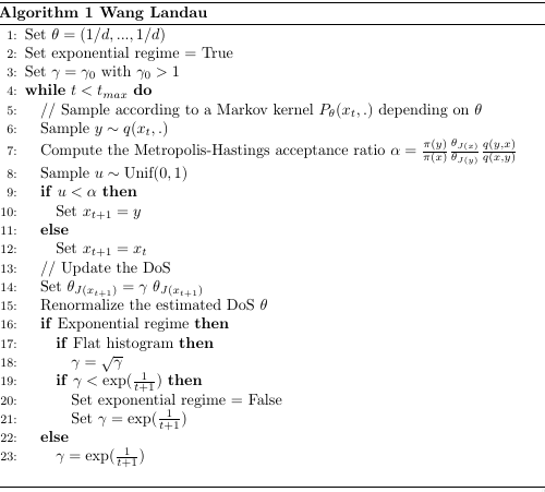
The WL algorithm iteratively construct a sequence of estimates for the unknown vector .
Let be the index of the stratum containing point Points sampled in a given stratum by WL at time follows the probability density
To do so, the main steps are (see pseudo-code):
(i) Using the current estimate , sample a point according to a Markov kernel whose invariant distribution is given by Eq. eq-wl-biased-density,
(ii) update using a learning rate , and
(iii) evolve according to two possible strategies known as the regime and the exponential regime. (This latter option comes from the fact that .)
We note that the exponential regime is governed by a flat histogram, which allows checking that all bins are visited evenly. Denoting be the number of samples up to iteration falling into the i-th stratum . The vector is said to verify the flat histogram (FH) criterion provided that, given a constant :
The Wang-Landau algorithm
Adaptivity
The previous algorithm uses a proposal to propose a novel sample/conformation from the current one .
This proposal is key to ensure that WL will diffuse across all strata.
Following [59], we resort to the notion of diffusivity across strata, using so-called aggregated transition matrices (ATM) and climbing times [59].
Consider an execution of WL. The aggregated transition matrix (ATM) for the proposal , denoted , is the row stochastic matrix providing the frequencies of transitions between strata corresponding to the moves proposed by along the execution. (Nb: column corresponds to moves ending outside the bounded region .)
The aggregated transition matrix for WL, denoted , is the row stochastic matrix providing the frequencies of transitions within WL.
Samples accepted are also used to measure the time taken to travel across all strata:
The climb across strata is defined by two times and such that
and .
and , .
The climbing time is then .
Main input and output
This said, running WL requires the following:
Physical system and proposal/move set.
Main output. The algorithm saves datas contained in the WL Data Structure a given times on a class called T_DS_snapshot. This data structure contains by default:
Bin ranges (useful if bins are added at runtime)
Estimated DoS
Proposal / move set data per bin – see below
The aggregated transition matrices and climbs/descents times
The climbing and descending times
The number of times the Flat Histogram criterion was reached
The algorithm mode (flat Histogram regime or 1/t regime)
The number of steps since the beginning of the algorithms
These pieces of information can be either saved at fixed intervals or at intervals that scales exponentially with time for log plots.
C++ code design
For each case
1. describe the system in a few sentences
2. describe the adaptation of the DS needed for this case
3. make the code accessible optionnally
4. provide some examples / picts
Main classes
The software package is divided into 5 major components:
Physical system.. The physical system , provided by the user, specifies the state space and the energy function. It may also provide the gradient of the energy function, if used in conjunction with move set requiring differential information.
Move set and its controller.. The move set/proposal provides the mechanism to generate a novel conformation given an existing one, and also provides transition probabilities used to ensure detailed balance. The move set works in close collaboration with its so-called controller – see below.
WL algorithm. The Wang Landau class SBL::GT::T_Wang_Landau is the core one, which glues all pieces together and delivers the DoS estimation. It relies in particular on the WL data structure, which stores bin ranges, additional pieces of information detailed below, and provides the bins management policy. To perform specific processing, like numerical integration, the user must defined a custom WL DS, by inheritance from the default (provided) one.
Helper classes for simulations.. We also provide the class SBL::GT::T_WL_Simulation , which encapsulates the main ingredients and eases the task of launching a simulation on a given physical system using a given proposal.
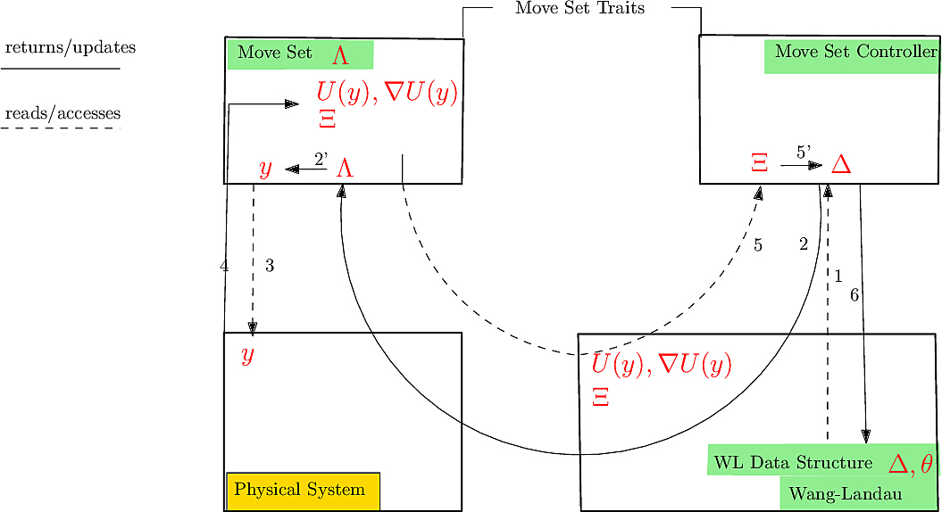
Data and data flow upon processing samples
To present the data exchange between the main components (Fig. fig-data-flow ), we introduce the following parameters and statistics:
: move set parameters (Class Move_Params ).
: statistics gathered during the generation of a novel conformation by the move set, and used to tune adaptivity (Class Move_Stats ).
: statistics, on a per bin basis, aggregating the observed values of along the simulation (Class Controller_Data ).
: DoS estimates.
Data flow and update of data structures upon generation of a point by the move set. Arrows indicate the ordering for data exchange between the main components. See [59] for details.
C++ use cases
Overview of main components
Physical System
A Physical system must define the following components:
a Conformation class that describes a point in state space
a compute_energy member function that computes the energy of a Conformation
a check_boundary_condition_fast function that checks if the conformation is still in state space (if you have constraints)
a check_boundary_condition_slow function that checks if the conformation is still in state space (if you have constraints), which will not be called every step of the algorithm (See rollback in paper)
a get_starting_sample that create an initial conformation
a Initial_Parameters class that will be passed to the constructor
OPTIONAL: if there is a non constant density/probability on your state space, define the density_ratio function that computes the density ratio between two conformation. See Boltzmann figure for an example.
The Conformation class must define:
a get_energy_function
a get_data function that returns what describes your conformation (so that the move set can move)
OPTIONAL: if you are using a move set that requires gradient: get_grad and get_grad_as_C_array
takes a Physical_System and Move_Set_Traits as template parameters
virtual class.
Virtual functions of T_WL_Simulation:
default provided: set_WL_general_parameters
default provided: set_WL_DS_parameters
set_physical_system_parameters
set_ms_controller_params
set_move_set_params
default provided: save_results
In addition, the library propose partial specialisation of T_WL_Simulation for the default move sets provided by the SBL that defines the set_ms_controller_params and set_move_set_params functions,
Then use the WL_Simulation helper class. First we specialize the Simulation class for our Physical System. This specialisation main role is to create initial bins of size 0.1 for energies in [0,1], and to give the dimension to the physical system.
class Isotrop_Energy_Well_Simulation_Combined: public Isotrop_Energy_Well_Simulation<Combined_MS_Traits>, T_WL_Simulation_Combined<Isotrop_Energy_Well_Physical_System>{
public:
using Base = T_WL_Simulation<Isotrop_Energy_Well_Physical_System,Combined_MS_Traits>;
using Base1 = Isotrop_Energy_Well_Simulation<Combined_MS_Traits>;
using Base2 = T_WL_Simulation_Combined<Isotrop_Energy_Well_Physical_System>;
The Ising model is discrete therefore a custom move set has to be defined. For this example, the WL_Simulation class will not be used since it was designed around the predefined continuous move sets. Besides, it allows us to see how to set up Wang_Landau for start to finish.
The ising model for a 2D grid:
periodic 2D grid of size LxL with lables + or - 1:
if a single vertex if fliped, the energy can be easily updated without computing the whole sum
Then we define a Move Set that only do flips. Since this is a symetric move ( i.e. the probability of going from A to B is the same than going from B to A), we can define the probability of going from A to B as 1 (the normalisation does not matter here, this term will be simplified in the Metrpolis criterion anyway). There is no adaptivity here so the Move Set controller is doing nothing.
struct Spin_Move_Params{
};
struct Spin_Move_Stats{};
template <class Conformation>
class Spin_Move_Set{//: public Move_Set_Base<Conformation,Gaussian_Move_Params>{
Finally we can define our Wang-Landau classes for L = 16:
using Move_Set_Traits = Spin_Move_Set_Traits;
using Physical_System = Spin_Physical_System<16>;
using WL_Ising = T_Wang_Landau<Physical_System,Move_Set_Traits>;
and launch the simulation:
struct Parameters{
uint64_t num_steps;
double flat_hist;
std::string output_prefix;
std::string get_filename(){
return "Ising_flat_hist_" + std::to_string(flat_hist)
+ ".txt";
}
};
void run(uint64_t num_steps,Parameters params){
WL_Ising::Parameters params_test_adaptative;
WL_Ising::Physical_systems_parameters params_phy;
WL_Ising::WL_DS_Parameters params_ds;
WL_Ising::MS_controllers_parameters ms_controller_params; //nothing to set here
WL_Ising::Move_Set_Parameters ms_params; //nothing to set here either
//bin management:
params_ds.base_ds_params.accept_new_bins = true;
params_ds.base_ds_params.energy_levels_continuous = false;
params_ds.base_ds_params.new_bins_size = 0.1;
//flat histogram:
params_ds.base_ds_params.histo_check_frequency = 100;
params_ds.base_ds_params.flat_histogram_threshold = params.flat_hist;
//here we show other parameters that can be set, but that can usually be left as default
params_ds.base_ds_params.gamma_0 = 0.1;
params_ds.base_ds_params.learning_rate = -1;
params_ds.base_ds_params.density_updater_type = 2;
//save parameters
params_test_adaptative.save_type = DoS_save_frequency_type::Log_scale;
params_ds.base_ds_params.save_events = false;
params_test_adaptative.save_rate = 1.01;
params_test_adaptative.debug_display_rate = 1000000;
params_test_adaptative.roll_back_check_frequency = 2000;
WL_Ising WL_instance(params_test_adaptative,params_ds,params_phy,ms_controller_params,ms_params);
WL_instance.run_WL(num_steps);
//save results
std::string filename = params.get_filename();
//last snapshot:
auto last_snap = WL_instance.get_snapshots()[WL_instance.get_snapshots().size()-1];
//utility class to serialze results
WL_stats_serializer serializer;
//save the final histogram
std::string histogram_filename = params.output_prefix+"histogram_" + filename;
serializer.save_histogram(histogram_filename,last_snap);
//save the connetivity graph
std::string connectivity_filename = params.output_prefix+"connectivity_" + filename;
serializer.save_connectivity(connectivity_filename,last_snap);
//save climbs and descents
std::string climbs_filename = params.output_prefix+"climbs_" + filename;
std::string descents_filename = params.output_prefix+"descents_" + filename;
serializer.save_climbs(climbs_filename,last_snap);
serializer.save_climbs(descents_filename,last_snap);
}
int main(int argc, char* argv[]){
namespace po = boost::program_options;
Parameters params;
po::options_description desc("Allowed options");
desc.add_options()
("help,h", "produce help message")
("num_steps,n", po::value<uint64_t>(¶ms.num_steps)->default_value(1000000), "number of steps")
("flat_hist", po::value<double>(¶ms.flat_hist)->default_value(0.1), "flat histogram threshold")
("output_prefix", po::value<std::string>(¶ms.output_prefix)->default_value(""), "prefix to put in front of output files")
;
po::variables_map vm;
po::store(po::parse_command_line(argc, argv, desc), vm);
po::notify(vm);
if (vm.count("help")) {
std::cout << desc << "\n";
return 1;
}
run(params.num_steps,params);
}
/home/fcazals/projects/proj-soft/sbl/Core/Wang_Landau/demos
Using executable  /user/fcazals/home/projects/proj-soft/sbl-install/bin/boltzmann_energy_single_well_figures.exe
Computing at the following temperatures: [0.05, 100000, 0.01, 0.1]
T = 0.05; repeat num 1 out of 2
T = 0.05; repeat num 2 out of 2
T = 100000; repeat num 1 out of 2
T = 100000; repeat num 2 out of 2
T = 0.01; repeat num 1 out of 2
T = 0.01; repeat num 2 out of 2
T = 0.1; repeat num 1 out of 2
T = 0.1; repeat num 2 out of 2
Data generation over
Nb: The Wang-Landau algorithm usually yields extreme answers when very few points are used (compared to the number of points needed for convergence) since it works in log scale. We can see this behavior here since we get a warning about invalid numerical values when trying to compute the median error. This is clearly visible in the plot itself as the error curves are missing values for steps < 10^4.
/usr/lib64/python3.7/site-packages/numpy/lib/function_base.py:3405: RuntimeWarning: Invalid value encountered in median for 341 results
  r = func(a, **kwargs)