|
Structural Bioinformatics Library
Template C++ / Python API for developping structural bioinformatics applications.
|
|
Structural Bioinformatics Library
Template C++ / Python API for developping structural bioinformatics applications.
|
Authors: F. Cazals and T. Dreyfus and D. Mazauric
![]()
This package package provides method to perform various comparisons of two samples energy landscapes, taking into account the location of local minima, their occupancy probabilities, and possible their connexsions as encoded in a transition graph.
Comparing two (sampled) energy landscapes is of interest in various settings, e.g., to assess the coherence of two force fields for a given system (atomic, coarse grained), to compare two related systems (e.g. a wild type and mutant protein), or simply to compare simulations launched with different initial conditions (and check whether the same regions in conformational space have been visited).
In comparing two landscapes, two categories of criteria are of interest, namely
features of the basins, in particular the local minima and their associated occupancy probabilities, called masses for the sake of genericity in the sequel.
This package provides methods to compare (sampled) energy landscapes, in two guises:
Earth Mover Distance: a comparison method exploiting solely the location of local minima, and the masses of the basins.
These functionalities are available in the programs 

Landscapes and vertex weighted TG. In the sequel, we assume that the energy landscape (EL) is coded in a compressed transition graphs, as defined in section Energy landscapes . We also assume that each vertex is endowed with a mass, typically the volume or the occupancy probability of its catchment basin. The reader is also referred to the package dedicated to the construction of transition graph, see Transition_graph_of_energy_landscape_builders .
In the following we provide two comparison methods: the first one deals with features of the basins only, while the second one additionally exploits the information on transitions.
Basins and their masses.Consider the basin 


For small systems, the mass of the system may be obtained by integrating the Boltzmann factor over the basin region, namely:

If minima are found by optimization (e.g., basin hopping), the 
If, on the other hand, the samples are obtained from a thermodynamic ensemble, as is typically the case for molecular dynamics and Monte Carlo procedures, Boltzmann weighting is automatically satisfied; the basin weight can correspondingly be estimated from the number of points 

Consider two landscapes, for which masses of the basins have been computed.
For the sake of exposure, we call these two landscapes the source landscape 


The local minima and the associated basins of the source landscape are denoted 


We also assume that the weights of the basins have been computed. Denoting these 


To compare the two landscapes, we use the earth mover distance [171] , which is a particular case of mass transportation [190] . Intuitively, the technique fills basins in the target (aka demand) landscape using mass from basins of the source landscape. A basin from 


Finding the optimal i.e. least cost transport plan amounts to solving the following linear program (LP):

The first equation is the linear functional to be minimized, while the remaining ones define linear constraints. In particular, the second one expresses the fact that every basin from 

Based on this linear program, we introduce the total number of edges, the total flow, the total cost, and their ratio, known as the earth mover distance [171] :

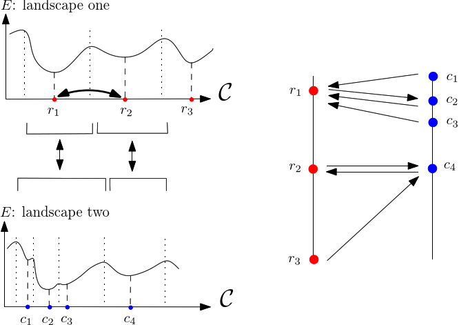 |
| Comparing two energy landscapes The landscape |
The previous comparison ignores transitions between local minima. To take these connections into account, we modify the method by imposing connectivity constraints to transport plans. To see whether a transport plan is valid, pick any connected subgraph 

An important remark is the following: a transport plan respecting connectivity constraints may not fully satisfy the demand. (It can actually be shown that there exist instance such that no transport plan fully satisfies the demand.)
Since EMD-CC does not necessarily admit a solution fully satisfying the demand, we define the problem Earth Mover Distance with Cost and Connectivity Constraints :
Note that the previous definition calls for two algorithms:
algorithm 


The latter algorithm actually has 2 recursion modes. To see which, assume that an interval ![$[0,C_{max}]$](form_559_dark.png)
Recursion mode: refined. Given two costs 


a) If the two total volumes of flow with cost ![$[C_{inf},C]$](form_563_dark.png)
![$[C,C_{sup}]$](form_564_dark.png)
Recursion mode: coarse. Similar to refined mode, except that only option b) is considered.
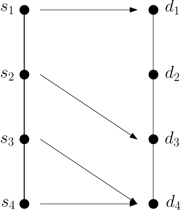 |
| The solution of the linear program may not satisfy connectivity constraints A transport plan between a source and a demand graph each consisting of a linear chain of four vertices. The vertices of the edge    |
In the following, we specify the two programs sbl-energy-landscape-comparison-euclid.exe and sbl-energy-landscape-comparison-lrmsd.exe, which differ by the type of metric used to compare distances between the points associated to vertices defining the graphs.
Main options.
Input.
Main output.
Optional output. Comments.
Once the weights of basins have been computed, solving the linear program of Eq. (eq-emd-lp) has polynomial complexity [118] . Practically, various solvers can be used, e.g. the one from the Computational Geometry Algorithms Library [55] , lp_solve, the CPLEX solver from IBM, etc. In the following, the algorithm solving the linear program of Eq. (eq-emd-lp) is called 
Finding transport plans respecting connectivity constraints turns out to be a hard combinatorial problem [42] . The problem is not in APX, which means that if 
Following definition def-tp-cc, we provide two algorithms:

Using the previous algorithm(s), in a manner analogous to Eq. (eq-emd-lp-dist), we define the total number of edges, the total flow, the total cost, and their ratio:


The programs of Energy_landscape_comparison described above are based upon generic C++ classes, so that additional versions can easily be developed.
In order to derive other versions, there are two important ingredients, that are the workflow class, and its traits class.
T_Energy_landscape_comparison_traits:
T_Energy_landscape_comparison_interface_workflow:
See the following jupyter notebook:
from SBL import SBL_pytools
from SBL_pytools import SBL_pytools as sblpyt
help(sblpyt)

from SBL import TG_weights_from_normalized_boltzmann
from TG_weights_from_normalized_boltzmann import *

from SBL import TG_builders
from TG_builders import *

from SBL import EMD_comparators
from EMD_comparators import *

from SBL import EL_comparators
from EL_comparators import *
The options of the compare method in the next cell are:
def cmp_landscapes(sbl_exe_name, tg1, tg2, lp_solver, symmetric, connectivityConstraints, plot_tp=False):
    odir = EL_comparators.compare(sbl_exe_name, tg1, tg2, lp_solver, symmetric, connectivityConstraints)

    EMD_comparators.scatter_plot_unit_cost_flow_DB(odir, "emd_engine.xml")
    if symmetric:
        EMD_comparators.scatter_plot_unit_cost_flow_DB(odir, "emd_engine_symmetric.xml")

    if (plot_tp):
        EMD_comparators.plot_transportation_plan(odir, "transportation_plan.dot")
        if symmetric:
            EMD_comparators.plot_transportation_plan(odir, "transportation_plan_symmetric.dot")
sbl_exe_name = "sbl-energy-landscape-comparison-euclid.exe"

tg1 = "data/himmelbleau_tg.xml"
tg2 = "data/himmelbleau_transition_graph_noisy.xml"

lp_solver = "clp"
symmetric = True
connectivityConstraints = False

cmp_landscapes(sbl_exe_name, tg1, tg2, lp_solver, symmetric, connectivityConstraints, True)


sbl_exe_name = "sbl-energy-landscape-comparison-euclid.exe"

tg1 = "data/himmelbleau_tg.xml"
tg2 = "data/himmelbleau_transition_graph_noisy.xml"


lp_solver = None # since EMD is used
symmetric = True
connectivityConstraints = True

cmp_landscapes(sbl_exe_name, tg1, tg2, lp_solver, symmetric, connectivityConstraints, False)
from SBL import TG_builders
from TG_builders import *

tg1 = TG_builders.build_transition_graph_fromDB("lrmsd",
                                    "data/bln69_database_minima_conformations_1.txt",\
                                    "data/bln69_database_minima_energies_1.txt",\
                                    "data/bln69_database_transitions_conformations_1.txt",\
                                    "data/bln69_database_transitions_energies_1.txt",\
                                    "data/bln69_database_transitions_1.txt",\
                                    "tmp-results-tg-1",\
                                    "data/bln69_database_minima_weights_1.txt")
print(tg1)
tg2 = TG_builders.build_transition_graph_fromDB("lrmsd",
                                                "data/bln69_database_minima_conformations_2.txt",\
                                    "data/bln69_database_minima_energies_2.txt",\
                                    "data/bln69_database_transitions_conformations_2.txt",\
                                    "data/bln69_database_transitions_energies_2.txt",\
                                    "data/bln69_database_transitions_2.txt",\
                                     "tmp-results-tg-2",\
                                    "data/bln69_database_minima_weights_2.txt")
print(tg2)
sbl_exe_name = "sbl-energy-landscape-comparison-lrmsd.exe"
tg1 = "tmp-results-tg-1/sbl-tg-builder-lrmsd__tg.xml"
tg2 = "tmp-results-tg-2/sbl-tg-builder-lrmsd__tg.xml"

lp_solver = "clp"
symmetric = True
connectivityConstraints = False

cmp_landscapes(sbl_exe_name, tg1, tg2, lp_solver, symmetric, connectivityConstraints, False)


#cmp_bln(lp_solver=None, symmetric=True, connectivityConstraints=True)
sbl_exe_name = "sbl-energy-landscape-comparison-lrmsd.exe"
tg1 = "tmp-results-tg-1/sbl-tg-builder-lrmsd__tg.xml"
tg2 = "tmp-results-tg-2/sbl-tg-builder-lrmsd__tg.xml"

lp_solver = None
symmetric = True
connectivityConstraints = True

cmp_landscapes(sbl_exe_name, tg1, tg2, lp_solver, symmetric, connectivityConstraints, False)


