|
Structural Bioinformatics Library
Template C++ / Python API for developping structural bioinformatics applications.
|
|
Structural Bioinformatics Library
Template C++ / Python API for developping structural bioinformatics applications.
|
![]()
Authors: A. Lheritier and F. Cazals
Comparing two sets of multivariate samples is a central problem in data analysis. From a statistical standpoint, one way to perform such a comparison is to resort to a non-parametric two-sample test (TST), which checks whether the two sets can be seen as i.i.d. samples of an identical unknown distribution (the null hypothesis, denoted H0).
Accepting or rejecting H0 requires comparing the value obtained for the test statistic used against a pre-defined threshold, usually denoted 
Effect size calculation: one wishes to assess the magnitude of the difference.
Effect size and feedback analysis are easy for one-dimensional data, as one may use the effect size associated with a Mann-Whitney U-test, or may perform a density estimation and compute some kind of distance (say the Mallows distance) between the obtained distributions. However, such analysis are more complex for multivariate data.
This package fills this gap, proposing a method based upon a combination of statistical learning (regression) and computational topology methods [40] . More formally, consider two populations, each given as a point cloud in 
Step 1: a discrepancy measure is estimated at each data point.
Step 2: a clustering of samples is performed. A cluster reported involves samples with significant discrepancy (threshold user-defined), which in addition are in spatial proximity.
 |  |
| (A) | (B) |
 |  |
| (C) | (D) |
 |  |
| (E) | (F) |
 | |
| (G) | |
| Method: input and main output. (A) Point clouds–here uniformly sampling two ellipsis. (B) Local Discrepancy on a scale 0-1 computed at each sample point. (C) Persistence Diagram associated with the sublevel sets of the estimated discrepancy (see text for details). (D) Simplified Disconnectivity Forest illustrating the merge events between sublevel sets. Note that four clusters stand out (the four legs of the tree). (E) Clustering: clusters identified on the disconnectivity forest, mapped back into the ambient space. Note that the green and blue clusters are associated with the red population, while the remaining two come from the blue population. (F) Effect Size Decomposition. The area under the dashed line represents the total effect size. The area under the continuous line is the maximum effect size possible. The area of each bar represents the contribution of each cluster to the effect size. (G) Discrepancy Cumulative Distribution. | |
We aim at modeling the discrepancy between two datasets 


In the first step, we assign a label to each set and we compute, for each sample point, a discrepancy measure based on comparing an estimate of the conditional probability distribution of the label given a position versus the global unconditional label distribution.
Divergence measures between distributions. To define our discrepancy measure, recall that the Kullback-Leibler divergence (KLD) between two probability densities 


with the conventions 

For two discrete distributions 


The Jensen-Shannon divergence (JSD) [135] allows one to symmetrize and smooth the KLD by taking the average KLD of 


Discrepancy measure. In taking the average in Eq. (eq-JSD), two random variables are implicity defined: a position variable 


In the sequel, we will consider the conditional and unconditional mass functions 


The connexion between the JS divergence and the previous (conditional) mass functions is given by [40] :
![$ \JSD{\densdX}{\densdY} = \int_{\Rnt^d} \densdZ{z} \divKL{\cpmf[\cdot][\rvp]}{\cpmf[\cdot]} dz $](form_419_dark.png)
The previous lemma shows that the JSD can be seen as the average, over 

![$ \deltaz \equiv \divKL{\cpmf[\cdot][\rvp]}{\cpmf[\cdot]}. $](form_424_dark.png)
The following comments are in order:


Taking for granted such an estimator (see section Discrepancy estimation for its effective calculation), we finally obtain an estimator for
![$ \deltazestim{n} \equiv \divKL{\cestimi{n}{\cdot}{\rvp}}{\cpmf[\cdot]} $](form_434_dark.png)
In practice, this estimate is computed using a regressor based on nearest neighbors, see section Discrepancy estimation . The number of neighbors used for each samples is set to 

Joint distribution compatible sampling. Practically, the sizes 

To ensure that balanced data sets are used in the estimation, we resort to random multiplexer generating samples 
The multiplexer halts when the data on one of the two data sets has been exhausted, and the resulting pairs are used to perform the estimation. Note that selected samples from the non exhausted data set may not be used, yielding some information loss. Therefore, we may repeat the process 


To describe the second step in simple terms–see [40] for the details, we refer to the so-called watershed transform used in image processing or topographical analysis, see Watershed image processing and Drainage basin. In a nutshell, given a height function, called the landscape for short in the sequel, the watershed transform partitions its into its catchment basins, with one basin for each local minimum.
To transpose these notions in our setting, we proceed in two steps. First, we build a nearest neighbor graph connecting the samples—e.g. we connect each sample to its 

On the landscape, we focus on samples whose estimated discrepancy is less than 


To recap, our analysis aims at:
Identifying samples with significant discrepancy.
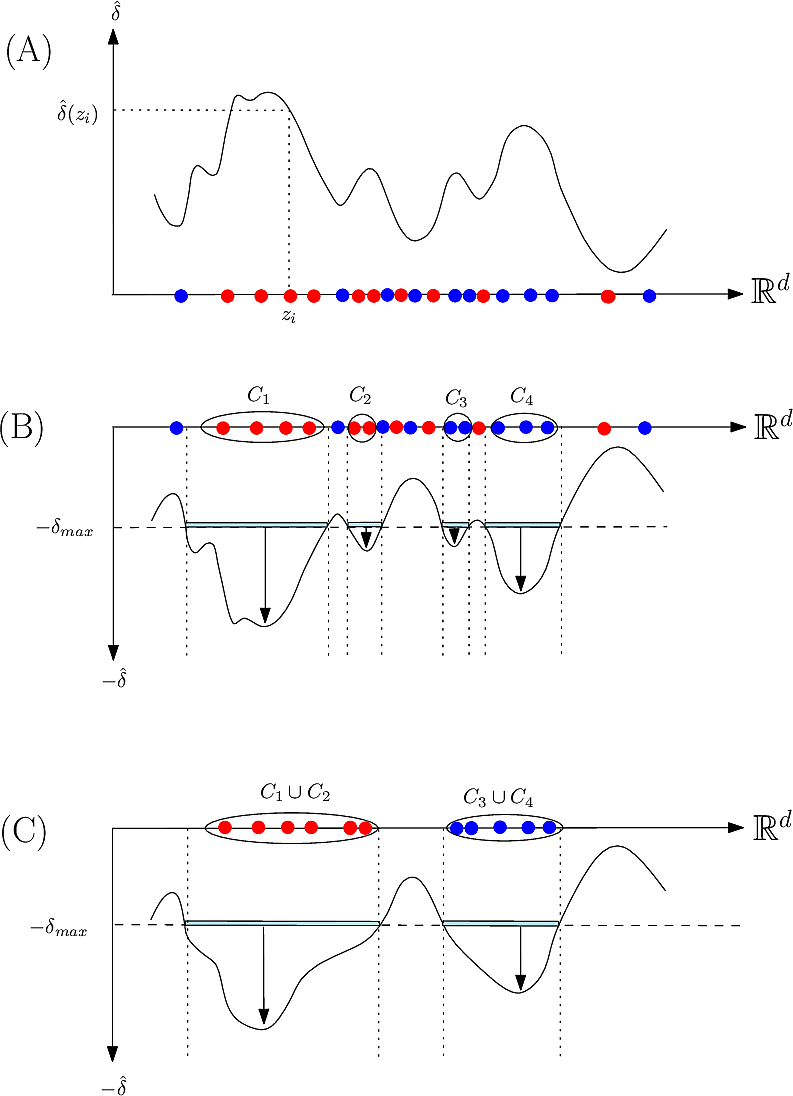 |
| Method: algorithm illustrated on a toy 1D example (A, discrepancy estimation) A discrepancy is estimated        |
This step consists of adding up the discrepancies on a per sample basis in a cluster 


Putting everything together, the program 
Persistence diagram: A plot showing for each minima a red cross with coordinates 
Discrepancy cumulative distribution function: The cumulative distribution function of the estimated discrepancies.
Disconnectivity forest: a hierarchical representation of the merge events associated with sublevel sets of the estimated discrepancy.
Clusters: A plot similar to the raw data plot, with one color per cluster. The points not belonging to any cluster are colored in gray.


For high dimensional date, we also provide the following 2D embeddings:
Raw data embedding: For samples embedded in 2D or 3D space, a plot of the points with a color to indicate the label (blue: 

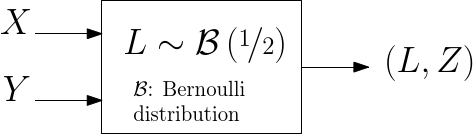 |
| Random multiplexer generating pairs (label, position). |
In the sequel, we specify the main steps and the options offered, see also Fig. fig-workflow-ddbc .
The first step is carried out by the python program
The script generates:
Main options:
Example:
> sbl-ddbc-step1-discrepancy.py -f data/ellipse_w_2_h_10_n_1000__X.dat -g data/ellipse_w_2_h_10_n_1000__Y.dat --theta0 0.5 --kofn-power 0.66 -B 1 --directory results
This step aims to provide a 2D embedding of the points, for visualization purposes. The embedding is obtained from Multi-dimensional scaling . While the default option consists of using the Euclidean distance to obtain the embedding, it is also possible to pass a more general distance matrix. Relevant such distances in the context of molecular modeling are the least Root Mean Square Deviation, as well as distances on the flat torus when dealing with internal coordinates. See the package Molecular_distances .
The corresponding plots may be used in the third step. It is carried out by the python program 
The script generates 3 files:
Main options:
Example:
> sbl-ddbc-2D-colored-embedding.py -f results/ellipse_w_2_h_10_n_1000__X_ellipse_w_2_h_10_n_1000__Y
The second step is carried out using the python program 

The script generates a number of files, the key ones being:
Main options:
Example:
> sbl-ddbc-step2-clustering.py -p results/ellipse_w_2_h_10_n_1000__X_ellipse_w_2_h_10_n_1000__Y.pointsWdim -w results/ellipse_w_2_h_10_n_1000__X_ellipse_w_2_h_10_n_1000__Y.heightDiv -n 6 -P --rho 0.1 --deltamax 0.1 -d results -o ellipse_w_2_h_10_n_1000__X_ellipse_w_2_h_10_n_1000__Y -v
The third step is carried out using the python program 
The script generates three images:
Main options:
Example:
> sbl-ddbc-step3-cluster-plots.py -f results/ellipse_w_2_h_10_n_1000__X_ellipse_w_2_h_10_n_1000__Y.vertices -c results/ellipse_w_2_h_10_n_1000__X_ellipse_w_2_h_10_n_1000__Y__sublevelsets_connected_components.xml -p results/ellipse_w_2_h_10_n_1000__X_ellipse_w_2_h_10_n_1000__Y.2Dpoints
In this section, we explain how to compute the estimator of Eq. (eq-deltaz), using the framework of regression [104] , and more precisely regressors based on


In the regression problem, the goal is to build an estimator 


In order to apply this framework to our problem, note that the correspondence 
![$ m(\rvp)=\cpmf[1][\rvp]. $](form_484_dark.png)
Then, we can use the following estimator for

Note that it is required that 
Using Eq. (eq-estim-pmflz), we finally obtain an estimator for

Precisely defining persistence is beyond the scope of this user manual, and the reader is referred to [89] , as well as to [40] for all details.
We comment on three issues, though:
Practically, our algorithm operates in a discrete setting wince the input consists of samples. The samples are used to build a nearest neighbor graph (NNG), by connecting each sample to a number of nearest neighbors (for a suitable distance metric), from which local minima and saddles can be identified [57] .
Equipped with a NNG, reporting the connected components (c.c.) of a sublevel set is a mere application of the so-called union-find algorithm, whose complexity is essentially linear in the number of samples processed. See [57] for details.
For large datasets though, in exploratory data analysis, the previous union-find algorithm may be called for varying values
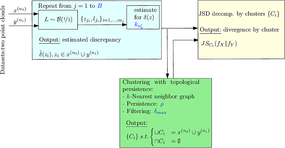 |
| Method: workflow. In blue: the parameters. |
The following two external dependencies are used in this applications:
See the following jupyter demos:
The options of the step1 method in the next cell are:
from SBL import SBL_pytools
from SBL_pytools import SBL_pytools as sblpyt
#help(sblpyt)
import re  #regular expressions
import sys #misc system
import os
import pdb
import shutil # python 3 only


def step1(odir, points1, points2, theta0 = 0.5, kofnPower = 0.66, resampling = 1):

    if os.path.exists(odir):
        os.system("rm -rf %s" % odir)
    os.system( ("mkdir %s" % odir) )

    # check executable exists and is visible
    exe = shutil.which("sbl-ddbc-step1-discrepancy.py")
    exe_opt = shutil.which("sbl-ddbc-2D-colored-embedding.py")

    if exe and exe_opt:
        print(("Using executable %s\n" % exe))
        cmd = "sbl-ddbc-step1-discrepancy.py -f %s -g %s --directory %s" % (points1, points2, odir)
        cmd += "  --theta0 %f --kofn-power %f -B %d > log.txt" % (theta0, kofnPower, resampling)
        print(("Running %s" % cmd))
        os.system(cmd)

        #sblpyt.show_log_file(odir)

        cmd = "ls %s" % odir
        ofnames = os.popen(cmd).readlines()
        prefix = os.path.splitext(ofnames[0])[0]

        cmd = "%s -f %s/%s" % (exe_opt, odir, prefix)
        print(("Running %s" % cmd))
        os.system(cmd)


        print("All output files:")
        print(os.popen(cmd).readlines())

        images = []
        images.append( sblpyt.find_and_convert("2Dembedding-discrepancy.png", odir, 100) )
        images.append( sblpyt.find_and_convert("2Dembedding-populations.png", odir, 100) )
        print(images)
        sblpyt.show_row_n_images(images, 100)
    else:
        print("Executable not found")
The options of the step1 method in the next cell are:
def step2(odir, ifn_points, ifn_weights, n = 6, P = True, rho = 0.1, deltamax = 0.1):
    # check executable exists and is visible
    exe = shutil.which("sbl-ddbc-step2-clustering.py")
    if exe:
        print(("Using executable %s\n" % exe))
        cmd = "sbl-ddbc-step2-clustering.py -p %s/%s -w %s/%s -d %s -v" % (odir, ifn_points, odir, ifn_weights, odir)
        cmd += " -n %d --rho %f --deltamax %f" % (n, rho, deltamax)
        if P:
            cmd += " -P"
        cmd += " > log.txt"
        print(("Running %s"  % cmd))
        os.system(cmd)

        cmd = "ls %s" % odir
        ofnames = os.popen(cmd).readlines()
        print("All output files:",ofnames)
        prefix = os.path.splitext(ofnames[0])[0]

        images = []
        images.append( sblpyt.find_and_convert("disconnectivity_forest.eps", odir, 100) )
        images.append( sblpyt.find_and_convert("persistence_diagram.pdf", odir, 100) )
        print(images)
        sblpyt.show_row_n_images(images, 100)
    else:
        print("Executable not found")
def step3(odir, ifn_vertices, ifn_clusters, ifn_points):
    # check executable exists and is visible
    exe = shutil.which("sbl-ddbc-step3-cluster-plots.py")
    if exe:
        print(("Using executable %s\n" % exe))
        cmd = "sbl-ddbc-step3-cluster-plots.py -f %s/%s -c %s/%s -p %s/%s > log.txt" % \
            (odir,ifn_vertices, odir, ifn_clusters, odir, ifn_points)
        print(("Running %s" % cmd))
        os.system(cmd)

        #log = open("log.txt").readlines()
        #for line in log:         print(line.rstrip())

        images = []
        images.append( sblpyt.find_and_convert("step3-2Dembedding-clusters.png", odir, 100) )
        images.append( sblpyt.find_and_convert("step3-bars.png", odir, 100) )
        images.append( sblpyt.find_and_convert("step3-discrepancy-cumulative-distribution.png", odir, 100) )
        sblpyt.show_row_n_images(images, 100)
        print(images)
    else:
        print("Executable not found")
print("Marker : Calculation Started")
odir_ellipsis = "exple-ellipsis"
step1(odir_ellipsis, "data/ellipse_w_2_h_10_n_1000__X.dat", "data/ellipse_w_2_h_10_n_1000__Y.dat")
print("Marker : Calculation Ended")

print("Marker : Calculation Started")
step2(odir_ellipsis, "ellipse_w_2_h_10_n_1000__X_ellipse_w_2_h_10_n_1000__Y.pointd",
      "ellipse_w_2_h_10_n_1000__X_ellipse_w_2_h_10_n_1000__Y.heightDiv")
print("Marker : Calculation Ended")

print("Marker : Calculation Started")
step3(odir_ellipsis, "ellipse_w_2_h_10_n_1000__X_ellipse_w_2_h_10_n_1000__Y.vertices",
      "sbl-Morse-theory-based-analyzer-nng-euclid__sublevelsets_connected_components.xml",
      "ellipse_w_2_h_10_n_1000__X_ellipse_w_2_h_10_n_1000__Y.2Dpoints")
print("Marker : Calculation Ended")

Another 2D example, with two populations of 2000 points, each drawn from a Gaussian mixture
the first population: 2000 points drawn according to a mixture of four spherical Gaussians with equal probability.
the second population: drawn according to a mixture of four non-spherical Gaussians with equal probability.
print("Marker : Calculation Started")
odir_gaussian = "exple-gaussian"
step1(odir_gaussian, "data/gaussianMixture6__d_2_n_2000_X.dat", "data/gaussianMixture6__d_2_n_2000_Y.dat")
print("Marker : Calculation Ended")

print("Marker : Calculation Started")
step2(odir_gaussian, "gaussianMixture6__d_2_n_2000_X_gaussianMixture6__d_2_n_2000_Y.pointd",
      "gaussianMixture6__d_2_n_2000_X_gaussianMixture6__d_2_n_2000_Y.heightDiv", deltamax=0.25)
print("Marker : Calculation Ended")

print("Marker : Calculation Started")
step3(odir_gaussian, "gaussianMixture6__d_2_n_2000_X_gaussianMixture6__d_2_n_2000_Y.vertices",
      "sbl-Morse-theory-based-analyzer-nng-euclid__sublevelsets_connected_components.xml",
      "gaussianMixture6__d_2_n_2000_X_gaussianMixture6__d_2_n_2000_Y.2Dpoints")
print("Marker : Calculation Ended")

In the following, we process 2 x 1600 points en dimension 784, from the MNIST dataset
An example illustrating the processing of real data in high dimension, we process a mixture of handwritten digits, each represented as an 28 x 28 gray-scale image -- see the MNIST dataset \cite lecun1998mnist .
The two populations see also \ref fig-digits-in-out , were chosen as follows:
blue population, 1600 digits: 100 digits 3, 500 digits 6, and 1000 digits 8.
red population, 1600 digits: 1000 digits 3, 500 digits 6, ans 100 digits 8.
print("Marker : Calculation Started")
odir_mnist = "exple-mnist"
step1(odir_mnist, "data/mnist368_100_500_1000_X.dat", "data/mnist368_1000_500_100_Y.dat")
print("Marker : Calculation Ended")

print("Marker : Calculation Started")
step2(odir_mnist, "mnist368_100_500_1000_X_mnist368_1000_500_100_Y.pointd",\
      "mnist368_100_500_1000_X_mnist368_1000_500_100_Y.heightDiv", n=30, deltamax=0.34)
print("Marker : Calculation Ended")

print("Marker : Calculation Started")
step3(odir_mnist, "mnist368_100_500_1000_X_mnist368_1000_500_100_Y.vertices",
      "sbl-Morse-theory-based-analyzer-nng-euclid__sublevelsets_connected_components.xml",
      "mnist368_100_500_1000_X_mnist368_1000_500_100_Y.2Dpoints")
print("Marker : Calculation Ended")
