|
Structural Bioinformatics Library
Template C++ / Python API for developping structural bioinformatics applications.
|
|
Structural Bioinformatics Library
Template C++ / Python API for developping structural bioinformatics applications.
|
![]()
Authors: N. Malod-Dognin and R. Andonov
Given a polypeptide chain, a protein contact map is a binary matrix such that the i-j-th element is one if the two corresponding 
In the CMO approach, the similarity between two proteins is determined by the extent of overlap of their contact maps.
See Protein Contact Map for more detail, and Fig. fig-CMO for an illustration.
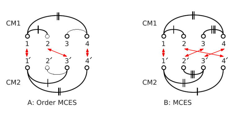 |
| Contact Map Overlap (A)Vertex set (1, 2, 4) from CM1 is matched with vertex set (1', 3', 4') from CM2. Common edges (two in this case) are denoted by the same number of vertical dashes. This is an order preserving MCES with maximum score 2. (B) Vertex set (1, 2, 3, 4) from CM1 is matched with vertex set (1', 4' , 2', 3') from CM2. This is a MCES with score 3. The order is not preserved. |
The formal definition of CMO is as follows. Let 

Under the alignment (matching, one-to-one map) 


The CMO problem is to find the optimal 

Apurva is a Contact Map Overlap maximization (CMO) solver. Given two protein structures represented by two contact maps, Apurva computes the amino-acid alignment that maximizes the number of common contacts. More information about the solver can be found in the articles [10] and [11] .
Apurva can process contact maps. A contact map file is divided in three sections, separated by an empty line.
The first section describes the contacts between the amino-acids. The first line contains an integer value X, which is the number of residues. Note that residues are labelled starting from one. The second line contains an integer value Y, which is the number of contacts. The next Y lines each contain two integer values i and j, i<j, the tail and head residues of each contact.
The second section describes the secondary structure assignment of the protein. It start with a line containing an integer value S, which is the number of secondary structure elements (SSE). It is then followed by S lines, each containing two integers (i and j) and a symbol t, where i is the first amino-acid of the SSE, j is the last amino-acid of the SSE, and t is the type of the SSE (either H for an alpha-helix, or b for a beta-strand).
The contact map files in the sequel were generated as follows: parameters:
Here is the contact map file for chain A in file 1vfb.pdb :
107
372
0 2
...
104 106

10
3 6 b
...
101 105 b
13
0 2 13
...
8 9 9
The first line indicates the number of residues, the second line the number of contacts, and then all contacts are enumerated by residue identifiers. After a blank line, the number of secondary structure elements (SSE) are indicated. Then, the start residue, the end residue, and the type of SSE (b for beta-sheet and H for alpha-helix). Finally, the number of contacts between SSE is followed by the SSE identifiers and the number of residues in contact between the two SSE.
CMO is an NP-hard problem [102] . The algorithms used here to solve CMO provided here are presented in [10] and [11] . These algorithms use an an integer programming model for CMO, and solve it with an an exact branch-and-bound algorithm with bounds obtained by a novel Lagrangian relaxation.
In this section, we present the executable 
Restrictions on PDB files.
Apurva can process .PDB files (.pdb or .ent), with the following restrictions:
Options.
Examples.
Apurva will align the two contact maps 1amkA.hcm and 1aw2A.hcm, and will display the corresponding alignment :
./sbl-apurva.exe --cm1 ./1amkA.hcm --cm2 ./1aw2A.hcm --display 2
Apurva will align chain A of 1amk.pdb with chain A of 1aw2.pdb, and will generate two files for VMD that highlight the matching between the two protein chains :
./sbl-apurva.exe --pdb1 1amk.pdb --chain1 A --pdb2 1aw2.pdb --chain2 A --vmd 1