Hamiltonian_Monte_Carlo

Authors: F. Cazals and A. Chevallier and S. Pion

Introduction

Sampling a high dimensional distribution $\pi(x)$ is a very challenging problem, in particular when the target distribution allocates its mass on a typical set of small dimension.

One efficient solution to deal with such cases is Hamiltonian Monte Carlo (HMC) [20] and [148] .

Based on a generic algorithm able to sample an isotropic Gaussian distribution $\pi(x) = \exp(- \|x\|^2 / (2\sigma_i^2))$ defined on a bounded open set [55], this package proposes an implementation for the particular case of a polytope $K \subset \Rd{n}$ and a Gaussian distribution target distribution $\pi$ .

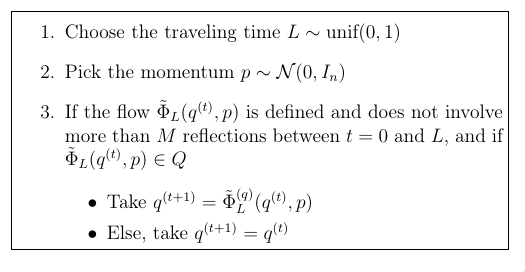
In a nutshell, the proposed method goes as follows:

Input: variance of the target Gaussian distribution $\pi$ , polytope, starting point.

Output: sequence of n points complying with the target density, in the interior of the polytope.

Algorithm and prerequisites

Algorithm

To sample a distribution $\pi$ in a high dimensional space, HMC defines a Markov chain in phase space $\Rd{2n}$ , with coordinates for the position , and coordinates for the velocity .

As the name suggests, HMC is governed by an ODE system defined by Hamilton’s equations. In a nutshell, a HMC step involves three steps which are (i) picking a random velocity p, (ii) traveling deterministically following Hamiltonian dynamic, and (iii) projecting down in configuration space.

A variant/extension of this algorithm was proposed in [55] , where reflexion on the boundary of the domain are used.

In our case, the distribution $\pi$ is a Gaussian centered at the origin of variance $\sigma$ , and exact trajectories are known for HMC.

In the sequel, we consider a polytope defined by linear inequalities, that is

$\begin{equation} A x \leq b. \end{equation}$

For the particular case of a polytope , reflexions are easily obtained from the intersection points with the hyper-planes bounding . This flow, illustrated on Fig. fig-hmc-step, is denoted as follow:

$\begin{equation} \begin{cases} \flowopr{t}:\overline K\times \mathbb R^n\rightarrow K\times \mathbb R^n\\ (q,p) \mapsto \flowopr{t}{q,p} \equiv ( \flowoprpos{t}{q,p} , \flowoprvel{t}{q,p} ). \end{cases} \end{equation}$

The overall algorithm is sketched on Fig. fig-algo.

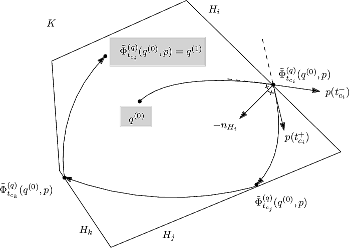The HMC algorithm: example trajectory staring at $q^{(0)}$ and ending at $q^{(1)}$

The HMC algorithm with reflexions on the boundary of the domain , taken to be a polytope in this package.

Numerics

In key issue in implementing geometric algorithms is robustness, as rounding operations may trigger erroneous evaluations and branching decisions.

As detailed in [55] , numerical robustness is ensured using multi-precision calculations, based on

The Lazy_exact_nt number type from CGAL.

the iRRAM library.. The released version of our code uses the following updated version of iRRAM.

Implementation and functionalities

This package provides the following program sbl-HMC-polytope-sampler.exe, whose main inputs are as follows:

Target Gaussian distribution $\pi$ : variance of the isotropic Gaussian. Note that we always assume that the Gaussian is centered at the origin.
Polytope specification as a linear system: CSV files for and to define the polytope $A x \leq b$ . (Nb: it is assumed that previous systems defines a bounded domain.)
Starting point:
- Ff no starting point provided, uses the origin $\transpose{(0,...,0)}$ as a default. Recall, though, that this point is expected to be in the interior of the convex.
- Otherwise, uses a starting point defined in a CSV file.
The number of samples to be generated in the interior of .

The starting point must be in the interior of the convex; if not, the program exits. (Nb: for a point on the boundary, one would have to check that the initial velocity is such that the trajectory enters the interior of the convex.)

C++ code design

Main components

The software package is divided into 3 major components:

HMC internal. The function SBL::GT::T_HMC_internal is a core function of this package: it computes the flow $\tilde{\Phi}_L$ (see the algorithm). However, it simply stops if the maximum number of reflection is reached, and it is up to the caller of the function to discard the result (this is done by the Polytope sampler class). Furthermore, this function takes a template parameter which describe the number type used and the associated functions required by SBL::GT::T_HMC_internal.

Kernels: double precision and multi-precision. Two kernels define all the necessary components required by HMC internal (such as function as cos, sin, etc) for different number types. These kernels are:

(File DP_Kernel.hpp) SBL::GT:Kernel_DP : kernel using a double as number type.

(File iRRAM_Kernel.hpp) SBL::GT::Kernel_iRRAM : kernel using iRRAM::REAL as number type.

The predicates and constructions used to ensure robustness are detailed in [55] .

Polytope sampler. SBL::GT::T_HMC_polytope_sampler is the class that should be used by users that still wishes to use C++ directly. It's constructor takes a CSV file for and , the variance $\sigma$ of the Gaussian, and an optional CSV file for the starting point. If no file is provided for the starting point, the point $\transpose{(0,...,0)}$ is used instead.

Dependency and compilation

As noted above, numerical robustness is ensured using multi-precision calculations, based on the iRRAM library.

The src directory of the package contains a CMakeList.txt file, which assume that iRRAM is installed in a directory referenced by the environment variable IRRAM_DIR. The pointed directory must contain sub-directories lib and include.

To generate the executable sbl-HMC-polytope-sampler.exe, one proceeds as follows:

cd sbl/Core/Hamiltonian_Monte_Carlo/src/Hamiltonian_Monte_Carlo
mkdir build
cmake ..
make

Matlab integration

The sampler can also be used from MATLAB. The corresponding code is provided in the directory Hamiltonian_Monte_Carlo/matlab .

To begin with, the program must be compiled using a MEX file. Open MATLAB in the directory Hamiltonian_Monte_Carlo/matlab and execute the following command to compile the MEX file:

mex HMC_Matlab.cpp CXXFLAGS="\$CXXFLAGS -std=c++17" -I${IRRAM_DIR}/include -L${IRRAM_DIR}/lib -liRRAM -lmpfr -lgmp

To use the MEX function, copy HMC_Matlab.mex* and libiRRAM.so to your working directory. The MEX function takes the following arguments (in this order)

starting position
starting velocity
matrix A describing hyperplanes
vector b describing hyperplanes
a parameter a that is determined by the variance of the Gaussian with $a = 1/(2*\sigma^2)$
travel time
max number of reflection

The following example shows how to sample a Cube in dimension 2.

%general parameters
dim=2;
a = 1;
travel_time = 1.5;
num_steps = 1000;

%starting point in a corner
x0 = zeros(dim,1);
for i = 1:dim
    x0(i) = 0.99;
end

%hyperplanes defining a cube
A = [1 0; -1 0 ; 0 1; 0 -1];
b = [1;1;1;1];

%saving results here
x_HMC = zeros(num_steps,dim);

%main loop
x_ = x0;
for i =1:num_steps
    u_ = randn(dim,1);
    [x_,u_] = HMC_Matlab(x_,u_,A,b,a,travel_time,100);
    x_HMC(i,:) = x_;
end

%plot result
scatter(x_HMC(:,1),x_HMC(:,2));

Examples

Cube in dimension 3

The linear systems involves one equation per face, whence the following:

Cube in dimension 3, matrix – see file demos/data/cube_dim3_A.csv:
```
1,0,0
0,1,0
0,0,1
-1,0,0
0,-1,0
0,0,-1
```

Cube in dimension 3, vector – see file demos/data/cube_dim3_b.csv:
```
1
1
1
1
1
1
```

Standard simplex in dimension 3

In this case, we need four equation:

Standard simplex in dimension 3, matrix – see file demos/data/stdsimplex_dim3_A.csv:
```
-1,0,0
0,-1,0
0,0,-1
1,1,1
```

Standard simplex in dimension 3, vector – see file demos/data/stdsimplex_dim3_b.csv:

Additionally, we may specify a starting point – see file demos/data/stdsimplex_dim3_p.csv:

0.001
0.001
0.001

Jupyter demo

See the following jupyter demos:

Jupyter notebook file
Hamiltonian_Monte_Carlo
Hamiltonian_Monte_Carlo¶

In the following, we illustrate the generation of samples within a polytope, according to a target Gaussian distribution¶
In [2]:

# http://www.open3d.org/docs/release/tutorial/Basic/pointcloud.html # http://www.open3d.org/docs/release/tutorial/Basic/working_with_numpy.html # http://www.open3d.org/docs/0.8.0/tutorial/Basic/visualization.html import os import numpy as np import open3d as o3d from open3d import JVisualizer from SBL_pytools import SBL_pytools as sblpyt # enclosing cube def line_set_cube(a): points = [[-a, -a, -a], [a, -a, -a], [-a, a, -a], [a, a, -a], [-a, -a, a], [a, -a, a], [-a, a, a], [a,a,a] ] lines = [[0, 1], [0, 2], [1, 3], [2, 3], [4, 5], [4, 6], [5, 7], [6, 7], [0, 4], [1, 5], [2, 6], [3, 7]] colors = [[1, 0, 0] for i in range(len(lines))] line_set = o3d.geometry.LineSet() line_set.points = o3d.utility.Vector3dVector(points) line_set.lines = o3d.utility.Vector2iVector(lines) line_set.colors = o3d.utility.Vector3dVector(colors) return line_set # enclosing cube def line_set_stdsimplex(a): points = [[0,0,0], [a, 0, 0], [0, a, 0], [0,0,a] ] lines = [[0, 1], [0, 2],[0,3],[1,2],[1,3],[2,3]] colors = [[1, 0, 0] for i in range(len(lines))] line_set = o3d.geometry.LineSet() line_set.points = o3d.utility.Vector3dVector(points) line_set.lines = o3d.utility.Vector2iVector(lines) line_set.colors = o3d.utility.Vector3dVector(colors) return line_set def process_case(model_name, dimension, sigma, num_samples, starting_point_file=None): A_file = "data/%s_dim%s_A.csv" % (model_name, dimension) b_file = "data/%s_dim%s_b.csv" % (model_name, dimension) ofname = "%s-dim%s-numsamples%s.xyz" % (model_name, dimension, num_samples) if (not os.path.isfile(A_file)) or (not os.path.isfile(b_file)): print("Check A and b files; exiting"); return; # generate the samples cmd = "sbl-HMC-polytope-sampler.exe -A %s -b %s -n %s -o %s" % (A_file, b_file, num_samples, ofname) cmd += " --sigma %s" % sigma if starting_point_file: cmd += " --starting_pt_file %s" % starting_point_file print(("Running %s" % cmd)) os.system(cmd) print("Done") if model_name == "cube": line_set = line_set_cube(1) elif model_name == "stdsimplex": line_set = line_set_stdsimplex(1) # generate the samples and directly visualize them if dimension == 3: pcd = o3d.io.read_point_cloud(ofname) #print(pcd) #print(np.asarray(pcd.points)) o3d.visualization.draw_geometries([pcd,line_set]) # generate the samples and pick the first three coordinates elif dimension > 3: data = np.loadtxt(ofname, usecols=[0,1,2]) #print(data) pcd = o3d.geometry.PointCloud() pcd.points = o3d.utility.Vector3dVector(data) o3d.visualization.draw_geometries([pcd,line_set])
Test in 3D: cube, standard simplex¶

The following call opens an interactive viewwer to inspect n=10000 samples in the 3D cube $[-1,1]^3$¶
To illustrate the role of the Gaussian width, we successively process two cases, namely $\sigma = 1$, and $\sigma = 0.1$. Static pictures also feature the enclosing cube.
In [7]:

process_case("cube", 3, 1, 10000)
Running sbl-HMC-polytope-sampler.exe -A data/cube_dim3_A.csv -b data/cube_dim3_b.csv -n 10000 -o cube-dim3-numsamples10000.xyz --sigma 1 Done
In [9]:

sblpyt.show_image("fig/cube-dim3-sig1-n10000.png")
In [5]:

process_case("cube", 3, 0.1, 10000)
Running sbl-HMC-polytope-sampler.exe -A data/cube_dim3_A.csv -b data/cube_dim3_b.csv -n 10000 -o cube-dim3-numsamples10000.xyz --sigma 0.1 Done
For the sake of visualization, here is a static picture of these samples¶
In [16]:

sblpyt.show_image("fig/cube-dim3-sig0dot1-n10000.png")
We now process the standard simplex $\{ x_i\geq 0, \sum_i x_i \leq 1\}$¶
To illustrate the role of the Gaussian width, we successively process two cases, namely $\sigma = 1$, and $\sigma = 0.1$ Static pictures also feature the enclosing simplex.
In [43]:

process_case("stdsimplex", 3, 1, 10000, "data/stdsimplex_dim3_p.csv")
Running sbl-HMC-polytope-sampler.exe -A data/stdsimplex_dim3_A.csv -b data/stdsimplex_dim3_b.csv -n 10000 -o stdsimplex-dim3-numsamples10000.xyz --sigma 1 --starting_pt_file data/stdsimplex_dim3_p.csv Done
In [11]:

sblpyt.show_image("fig/stdsimplex-dim3-sig1-n10000.png")
In [12]:

process_case("stdsimplex", 3, 0.1, 10000, "data/stdsimplex_dim3_p.csv")
Running sbl-HMC-polytope-sampler.exe -A data/stdsimplex_dim3_A.csv -b data/stdsimplex_dim3_b.csv -n 10000 -o stdsimplex-dim3-numsamples10000.xyz --sigma 0.1 --starting_pt_file data/stdsimplex_dim3_p.csv Done
In [17]:

sblpyt.show_image("fig/stdsimplex-dim3-sig0dot1-n10000.png")
Tests in higher dimension: cube in dimension 10¶

The first call generatessamples, and opens an interactive coordinate for the projection of the generated samples in 3D

The static figure is a capture of the latter
In [32]:

process_case("cube", 10, 1, 10000)
Running sbl-HMC-polytope-sampler.exe -A data/cube_dim10_A.csv -b data/cube_dim10_b.csv -n 10000 -o cube-dim10-numsamples10000.xyz --sigma 1 Done
In [15]:

sblpyt.show_image("fig/cube-dim10-sig1-n10000.png")

Table of Contents

Hamiltonian_Monte_Carlo

Introduction

Algorithm and prerequisites

Algorithm

Numerics

Implementation and functionalities

C++ code design

Main components

Dependency and compilation

Matlab integration

Examples

Cube in dimension 3

Standard simplex in dimension 3

Jupyter demo

Hamiltonian_Monte_Carlo¶

In the following, we illustrate the generation of samples within a polytope, according to a target Gaussian distribution¶

Test in 3D: cube, standard simplex¶

The following call opens an interactive viewwer to inspect n=10000 samples in the 3D cube $[-1,1]^3$¶

For the sake of visualization, here is a static picture of these samples¶

We now process the standard simplex $\{ x_i\geq 0, \sum_i x_i \leq 1\}$¶

Tests in higher dimension: cube in dimension 10¶