|
Structural Bioinformatics Library
Template C++ / Python API for developping structural bioinformatics applications.
|
|
Structural Bioinformatics Library
Template C++ / Python API for developping structural bioinformatics applications.
|
We present various data types used within the SBL.
The PDB format is widely used. The following molecular systems are used in several places, for testing / illustration purposes:
The potential energy of a molecular system is defined from a force field. In the SBL, all force fields are handled in a coherent way – see package Molecular_potential_energy .
Force field parameters are specified in a XML file – see the FFXML format from the OpenMM library. We provide XML files for the force fields used within the SBL :
Space filling models are defined from union of balls, see Terminology and Concepts and the corresponding applications Space Filling Models – Work Package: Space Filling Models .
The following are used to define / illustrate such data.
The atomic group radii define different sets of radii for the atoms. They are used as annotations of atoms from the pacakge ParticleAnnotator and are particularly important when particles (atoms or residues) are represented by 3D balls. The SBL provides three particular groups radii borrowed from ESBTL:
A number of algorithms are purely geometric and can be used without any biophysical semantic. For these cases, the following family of balls has been used for testing purposes:
Conformational analysis focus on the space describing molecular conformations, and the associated energy landscapes – see Terminology and Concepts .
In the following, we provide landscapes defined by mathematical functions, and also data related to specific molecular systems. The interested user is also referred to the comprehensive Cambridge Energy Landscape Database
This section briefly presents selected landscapes used to test our sampling algorithms.
As a simple illustration, we use the Himmelblau function, see Fig. fig-himmelblau and also Himmelblau's function on Wikipedia.
 |
| The Himmeblau function |
Function value. The function value is a degree two bivariate polynomial:

Gradient. Easily computed by hand.
Movet set to generate a new sample. To generate a new conformation, one picks a random conformations at a predefined distance 
The Rastrigin function is a classical non convex function used in optimization benchmarks.
Function value. Denoting 

.
Gradient. Easily computed by hand.
Movet set to generate a new sample. To generate a new conformation, one picks a random conformations at a predefined distance
The trigonometric terrain is a more complex function [163], challenging exploration algorithms in the 2D case, see Fig. fig-termino-trigo-terrain .
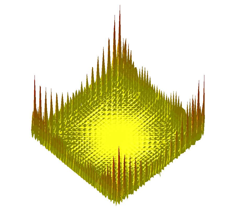 |
| The Trigonometric terrain function |
Function value. The function value is :

Gradient. Computed by hand.
Movet set to generate a new sample. To generate a new conformation, one picks a random conformation at a predefined distance
Model. To illustrate our sampling algorithms, we use a 69 residue BLN model protein [32] , whose landscape has been extensively sampled [188], [140] .
The BLN model represents each protein residue as one of 3 types of beads, namely hydrophobic(B), hydrophilic(L) and neutral(N).
Potential energy. The potential energy of the BLN69 model is given by:
![\begin{align}V = \frac{1}{2} K_r \sum_{i}^{N-1} (R_{i,i+1} - R_\text{e})^2
+ \frac{1}{2} K_\theta \sum_{i}^{N-2} (\theta_{i} - \theta_\text{e})^2
\\ + \epsilon \sum_{i}^{N-3} [A_i (1 + \cos \phi_{i}) + B_i(1 + \cos 3\phi_{i})]
\\ + 4 \epsilon \sum_{i}^{N-2} \sum_{j=i+2}^{N} C_{i,j} [ (\frac{\sigma}{R_{i,j}})^{12} - D_{i,j} (\frac{\sigma}{R_{i,j}})^6 ].
\end{align}](form_1095_dark.png)
Note that the first three terms are bonded terms, while the fourth is the non bonded term (Lennard-Jones potential). Parameter definitions and values are as specified in [188] .
Gradient. To compute the gradient of expression eq-bln-potential , we use the automatic differentiation tool 
Move sets to generate new conformations. A move set is a unitary operation thanks to which a new conformation is generated from a given conformation, typically at a predefined distance called the step size denoted
Three classical movesets, illustrated here for BLN69, are the following ones:
global moveset: the new conformation is chosen uniformly at random on the sphere of radius
interpolation moveset: the new conformation is chosen (uniformly at random) on the line-segment joining two conformations.
For the sake of clarity, let us detail the atomic move set. Denoting 


![$[0,1]$](form_322_dark.png)
![$[-1,1]$](form_1100_dark.png)

Note that in applying such a move set, the RMSD between the old and the new conformations is equal to
 |
| Example conformation of the BLN69 model The three types of beads are represented as follows: hydrophobic (B) in red, hydrophylic (L) in blue, and neutral (N) in green. Note the formation of a hydrophobic core clubbing the hydrophobic |
Transition graph connecting minima and saddles.
Conformations are central in applications from the Conformational Analysis group. Knowing minima and saddles in the conformational space elevated by the potential energy is important for testing the algorithms. A set of 458082 minima linked by 378913 saddles of BLN69 is available here. They were originally generated by Wales using a Basin Hopping algorithm. The archive is composed of 5 files :