|
Structural Bioinformatics Library
Template C++ / Python API for developping structural bioinformatics applications.
|
|
Structural Bioinformatics Library
Template C++ / Python API for developping structural bioinformatics applications.
|
Authors: F. Cazals and T. Dreyfus and S. Loriot
![]()
Surface areas and volumes of molecular models are fundamental quantities in structural bioinformatics. Two widely used models are the van der Waals model and the solventaccessible models". The programs of Space_filling_model_surface_volume compute the surface area and the volume of a model defined by a union of balls, following the two aforementioned models. The underlying algorithm partitions the volume into the restrictions of the balls to their respective Voronoi cells [43] , exploiting properties of the  -complex of the balls. Two points need to be stressed.
Surface area and volume computations are numerically challenging, due to the geometric constructions involved . Unlike all previous approaches which have systematically used fixed precision floating point (FP) calculations, programs of Space_filling_model_surface_volume use advanced numerics (interval arithmetic and calculations on degree two algebraic numbers) to certify the surface areas and volumes reported. That is, all results are returned in the form of an interval of FP numbers, which is certified to contain the true result. This strategy has been used to shown that (i) calculations based solely on FP numbers systematically incur errors — of typically 20%, and (ii) that the running time overhead of applications of Space_filling_model_surface_volume is of about two.
The computation of restrictions being based on the -complex of the balls processed, it is possible to compute along the way information on cavities of the model.
To recap, the main features of Space_filling_model_surface_volume are as follows:
Calculation of surface areas and volumes for a whole molecular model, or on a per ball basis – see package Union_of_balls_surface_volume_3. For the particular case of an atomic model of a protein, surface areas and volumes are also reported on a per residue level.
Calculation of the Betti numbers 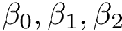 of the union of balls, which respectively characterize the number of connected components, the number of tunnels, and the number of cavities (i.e. pockets inside the molecule) – see package Betti_numbers.
Dissection of the surface area into its connected components. In particular, for a connected molecule, the surface areas of the cavities are returned – see package Union_of_balls_surface_volume_3.
Computation of the volume of the cavities, if any – see package Union_of_balls_surface_volume_3.
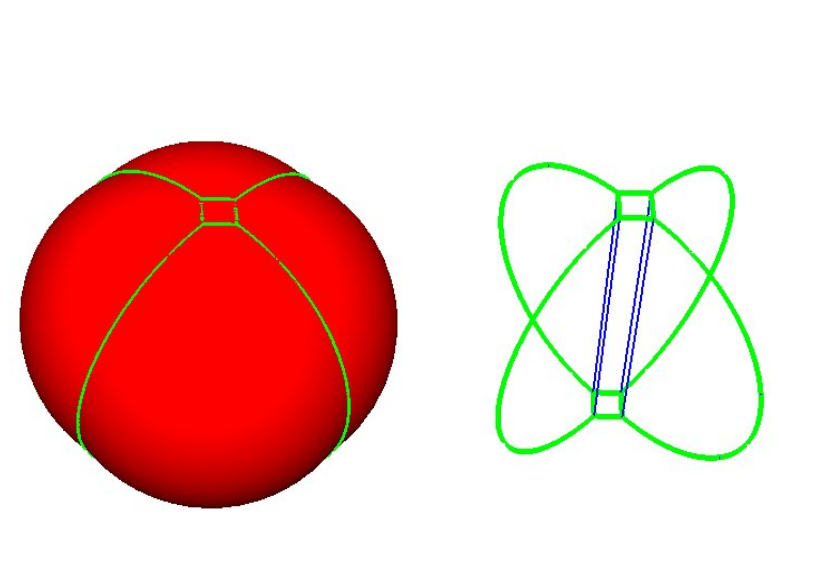 |
A union of five balls in 3D. This union decomposes into five restrictions, each bounded by spherical caps and planar faces. The 1-skeleton of the restrictions are represented by green curves. |
We consider a collection of  balls, namely
  . We assume that the coordinates of the center, and the radius of each ball are rational numbers. We wish to compute the volume of the domain
  , as well as the surface area of its boundary
  .
.
We denote  the Voronoi region of ball
  in the Voronoi (power) diagram of the balls, and we define the restriction
  of the ball as its intersection with its Voronoi region, that is
  . A restriction is termed exposed if it contributes to the boundary of the union.
As proved in [43] and illustrated on Fig. Restrictions, it is sufficient to compute restrictions to report surfaces and volumes:
These facts also account for the difficulty of computing surfaces and volumes, from a numerical standpoint. To understand why, it should be observed that two types of points are found on the boundary of a restriction:
found at the intersection of three spheres. The coordinates of these points are degree two algebraic numbers.The coordinates of these points appear in the formulae for the volume and surface area of a restriction, whence the need to compute them accurately. In a nutshell, these points can be handled in two ways, namely using interval arithmetic or using exact number types (rational numbers or algebraic numbers). The former is a fast strategy providing coarse approximations of the coordinates, while the latter provides more precise approximations, at the cost of more intensive calculations. Combining these strategies, we define the following three levels of precision:
In any case, a surface area or a volume is returned as an interval certified to contain the exact unknown value. See [43] for the typical width of these intervals.
Input. The main input of  is a molecular structure loaded from a PDB file. In this case, the library is used for deducing the set of balls corresponding to the molecule. Various options are available for tunning the set of balls representing the molecule (see the class SBL::Models::T_PDB_file_loader). Note that a default radius of
  is added to all atoms to define the Solvent Accessible Model of the input molecule.
Main options.
are:-f string: PDB file of the molecule to coarse grain–boundary-viewer string(=none): create a file for visualizing the boundary arcs with vmd or pymol-E: switch to more exact but longer calculations
Main output.
The files generated are:
For visualizing the halfedges of the boundary, we recommend you to install VMD (see the VMD web site): first load the input PDB file, then load the output visualization state files. The loading of visualization state files may be long, but is a lot faster using the fastload VMD script delivered with the library (in the scripts/vmd directory).
Input. The main input of  is a collection of balls from which the (power) Voronoi diagram will be computed. The file format used is a text file listing the balls (x y z radius).
Main options.
are:-f string: file listing the input family of 3D balls–boundary-viewer string(=none): create a file for visualizing the boundary arcs with vmd or pymol-E: switch to more exact but longer calculations
Main output. Identical to the PDB mode – except that the file on a per residue basis is not reported.
Remarks.
The SBL provides VMD and PyMOL plugins to use the programs of Space_filling_model_surface_volume . The plugins are accessible in the Extensions menu of VMD or in the Plugin menu of PyMOL . Upon termination of a calculation launched by the plugin, the following visualizations are available:
The new command "sbl_vorlume" is also defined: given a selection of atoms, it returns the volume and the solvent accessible surface area of this selection. For the sake of illustration, let us assume that the selection consists of all atoms. For VMD, the syntax is:
> sbl_vorlume [atomselect top "all"]
For PyMOL, the syntax is:
> sbl_vorlume("all")
The programs of Space_filling_model_surface_volume described above are based on generic C++ classes, so that additional versions can easily be developed.
In order to derive such versions, there are two important ingredients: the workflow class and the traits class.
T_Space_filling_model_surface_volume_traits:
T_Space_filling_model_surface_volume_workflow:
See the following jupyter demos:
We proceed as follows, using as an example PDB id 1vfb.pdb:
Note that statistics on a per atom basis are dumped in an xml file. A finer exploitation of these statistics on a per atom basis is provided below.
import re  #regular expressions
import sys #misc system
import os
import pdb
import shutil # python 3 only

#input filename  and output directory
ifname = ".././../../demos/data/1vfb.pdb"
odir = "results"
if not os.path.exists(odir):
    os.system("mkdir results")

# check executable exists and is visible
exe = shutil.which("sbl-vorlume-pdb.exe")
print( ("Using executable %s\n" % exe) )

# run command
cmd = "sbl-vorlume-pdb.exe -f %s --directory %s --verbose --output-prefix --log --boundary-viewer vmd" % (ifname,odir)
os.system(cmd)

# list output files
cmd = "ls %s" % odir
ofnames = os.popen(cmd).readlines()
print("\nAll output files:",ofnames)

# find the lof file and display log file
cmd = "find %s -name *log.txt" % odir
lfname = os.popen(cmd).readlines()[0].rstrip()
print("\nLog file is:", lfname)
#log = open(lfname).readlines()
# for line in log:         print(line.rstrip())
We now use the package PALSE , see https://sbl.inria.fr/doc/PALSE-user-manual.html , to collect all volumes and surface areas, on a per atom basis.
from SBL import PALSE
from PALSE import *

# create a DB of xml output files
database = PALSE_xml_DB()
database.load_from_directory("results",".*volumes.xml")

# from the XML files, retrive the  volume of atomic restrictions and compute the average
volumes = database.get_all_data_values_from_database("restrictions/item/total_volume", float)
volumes = PALSE_DS_manipulator.convert_listoflists_to_list(volumes)
ave_volume = sum(volumes)/float(len(volumes))
print( ("Average volume of atomic restrictions: %s" % ave_volume) )

# from the XML files, retrive the  surface areas of atomic restrictions and compute the average
areas = database.get_all_data_values_from_database("restrictions/item/total_area", float)
areas = PALSE_DS_manipulator.convert_listoflists_to_list(areas)
ave_area = sum(areas)/float(len(areas))
print( ("Average surface area of atomic restrictions: %s" % ave_volume) )
The list of areas can be used to inspect the distribution of surface areas on a per atom basis:
import matplotlib.pyplot as plt
import numpy as np

plt.hist(areas, density=1, bins=30)
plt.xlabel('Areas')
plt.ylabel('Probability')

Likewise, one can plot the distribution of volumes of Voronoi restrictions:
plt.hist(volumes, density=1, bins=30)
plt.xlabel('Areas')
plt.ylabel('Probability')
