|
Structural Bioinformatics Library
Template C++ / Python API for developping structural bioinformatics applications.
|
|
Structural Bioinformatics Library
Template C++ / Python API for developping structural bioinformatics applications.
|
![]()
Authors: F. Cazals and A. Commaret and L. Goldenberg
Let a parametric cluster model be a cluster model depending on parameters to be estimated. As opposed to clusters defined with respect to points, such as in k-means or k-medoids, parametric cluster models aim at providing insights on the geometry of the point set modeled.
This package presents the first method to compute spherical clusters [cazals2026modeling] , which were introduced in the context of subspace clustering [196] .
As illustrated by the logo of this package, a spherical cluster is defined by a ball, based on
See also Fig. fig-CM-examples-Iris for spherical clusters obtained on the classical Iris 4D dataset, and the sections below for the precise mathematical definitions.
   |
Spherical cluster models for the three clusters of the classical Iris 4D dataset: (Left) Setosa (Middle) Versicolor (Rigth) Virginica. Spherical cluster models for  |
Cluster identification as an optimization problem. Let 


Take 


Cluster optimization is concerned with the identification of the optimal parameters in the following sense:
Cluster optimization. Let

Spherical clusters. Recall that the unbiased variance estimate for distances within cluster 

To define the spherical cluster model [196] , also recall that the power of a point 


We define:
![$\eta \in ]0,1[$](form_1461_dark.png)


The rationale of this definition is that one wishes to find the center covering as many inliers as possible while minimizing the cost of outliers–points outside the spherical cluster.
Thus, the spherical cluster model depends both on inliers and outliers.
For a fixed data set

To study the previous function, for each 

so that one gets

The following is proved [cazals2026modeling] :
Theorem. (Strict convexity of 


While this theorem establishes the uniqueness of the SC center, the main difficulty to compute it is that the functional to be minimized is not smooth, see Fig. fig-opt-codim.
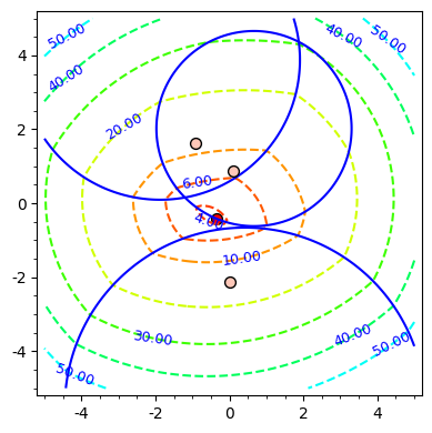  |
| Minima of |
An exact solver for spherical clusters, denoted 

and constructs a finite sequence of points 

This algorithm relies on three sub-routines called 


The reader is referred to [cazals2026modeling] for the details.
While the functional to be optimized in not smooth, it is known that BFGS works well in practice for non-differentiable functions [133].
We challenge 


Our algorithm is implemented in python and numpy. The reader is referred to [cazals2026modeling] for a detailed discussion of numerics and genericity assumptions.
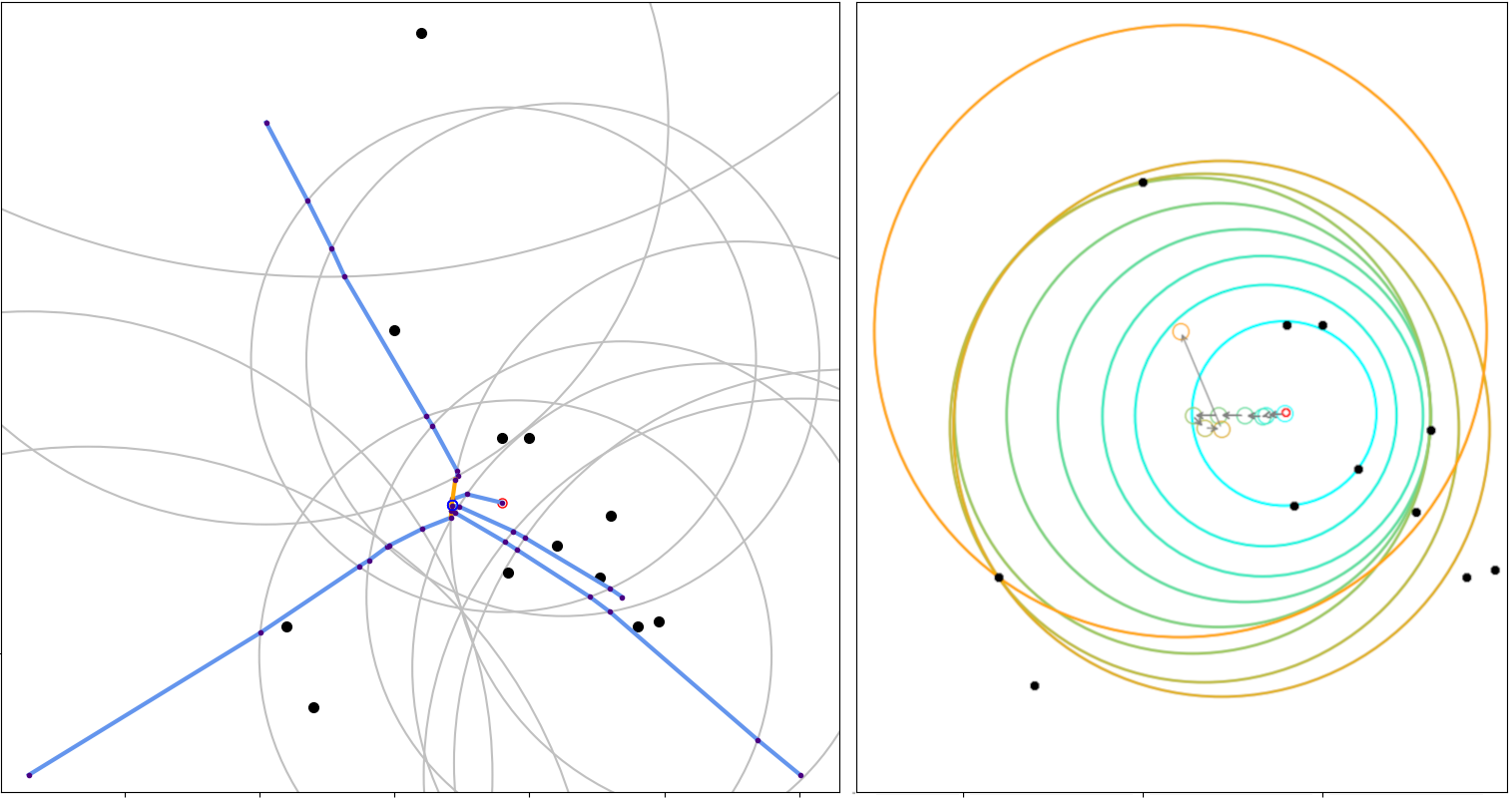 |
Spherical cluster: illustrations on a toy 2D dataset. (LEFT) Trajectories from five different starting points, with   |
Modeling point clouds with the SC model requires varying


The provided script sbl-sc-model.py implements two modes:
Main options. The main options of the script sbl-sc-model.py are as follows:
Single file mode. Fitting a SC model on one or several files, for one or several values of
sbl-sc-model.py --ifpaths iris_setosa.txt iris_versicolor.txt iris_virginica.txt --eta .3 .5 .7 --odpath results-Iris-4D
The calculation delivers a projection plot files, together with an xml file. Here is the output for virginica subset of the Iris-4D dataset, with 
<statistics>
<fname>iris_virginica</fname>
<n>50</n>
<d>4</d>
<algo-xBFGS>BFGS</algo-xBFGS>
<mu>1</mu>
<eta>0.5</eta>
<Exact-converged>True</Exact-converged>
<Exact-sanity>True</Exact-sanity>
<Exact-value>26.24517843427694</Exact-value>
<Exact-R2>0.4482605447117279</Exact-R2>
<Outlier-SESC-ave-cost>0.8466186591702239</Outlier-SESC-ave-cost>
<Outlier-SESC-num>31</Outlier-SESC-num>
<Outlier-COM-ave-cost>0.8207792662258733</Outlier-COM-ave-cost>
<Outlier-COM-num>50</Outlier-COM-num>
<Exact-time>0.04823482397478074</Exact-time>
<xBFGS-value>26.245178434277097</xBFGS-value>
<xBFGS-R2>0.4482605489741717</xBFGS-R2>
<xBFGS-time>0.02992666099453345</xBFGS-time>
<Ratio-values-exact-xBFGS>0.999999999999994</Ratio-values-exact-xBFGS>
<Ratio-time-exact-xBFGS>1.6117676470352489</Ratio-time-exact-xBFGS>
<Distance-exact-xBFGS>9.967294856861747e-08</Distance-exact-xBFGS>
<Distance-exact-PM>0.13782260415531594</Distance-exact-PM>
<traj-segments><LINEDESCENT>5</LINEDESCENT></traj-segments>
</statistics>
Multiple files mode. Assume that the directory $DATASET contains a list of clusters in txt format, and that the file $DATASET/clusters.txt lists these individual clusters by filename (Nb: filename not filepath). The calculations and statistics are easily obtained as follows:
sbl-sc-model.py -F $DATASET/clusters.txt --etag 0.1 --bfgs bfgs --odpath $DATASET/results-bfgs
sbl-sc-model.py -F $DATASET/clusters.txt --idpath $DATASET/results-bfgs --dsname MyDataset
The python implementation of [cazals2026modeling] provides the following modules / classes.
Solvers and associated statistics. The package proposes three solvers handling the non-smooth convex optimization introduced in [cazals2026modeling] :
These solvers make a consistent use of the class SBL::SESC_tools::SESC_tools , which provides various geometric calculations involved in the definition of the optimization problem.
Spherical cluster model. The class SBL::SESC_model::SESC_model serves as a data class to store all relevant pieces of information for a spherical cluster. This class itself relies on :
Large scale experiments. To compute spherical cluster models of collections of datasets (each given as a 
Visualization in 2D. As mentioned above, the –cells options triggers the dump of a trajectory file – .npz suffix. To ease our understanding of the spherical cluster model, the class SBL::SESC_visu::SESC_visu provides two visualization modes in 2D, which exploit these trajectory files:

Main script: sbl-sc-model.py. The design of this script follows the framework proposed in the package Script_design. The Spherical cluster model can be confronted to other cluster analysis provided in the package Cluster_analysis.