|
Structural Bioinformatics Library
Template C++ / Python API for developping structural bioinformatics applications.
|
|
Structural Bioinformatics Library
Template C++ / Python API for developping structural bioinformatics applications.
|
Authors: F. Cazals and T. Dreyfus ![]()
In the sequel, we consider a molecular structure associated with a molecular system Molecular_system and possibly the associated labels MolecularSystemLabelsTraits.
In the simplest case, each system corresponds to one partner in a complex. In a more general setting, as we shall see, a system provides a hierarchical decomposition of a partner. Note that the notion of system is oblivious to the precise geometric representation: in short, a system is defined by a collection of balls, which may be atoms or pseudo-atoms. For the sake of generality, these balls are called particles. At this stage, we just notice that when the particles represent atoms, the geometric model used is the solvent accessible model.
In this context, Space_filling_model_interface is a package of applications computing a parameter free representation of macro-molecular interfaces between systems, based on the 
These features are bound to two geometric constructions, namely the Voronoi diagram of the particles, and the associated
Space_filling_model_interface is based on generic c++ code, so that new applications are easily obtained for specific biophysical models, e.g. for specific atomic or coarse-grain models. By default, the following atomic resolution applications of Space_filling_model_interface are provided:


Applications of Space_filling_model_interface for coarse-grain models with one or two pseudo-atoms per residue is also provided.
In this section, we model the interaction between two partners 


The input is assumed to be a high resolution crystal structure of the complex, so that the particles represent atoms, using their atomic group radii. We represent this atomic structure by its solvent accessible model, that is, the radius of each particle is enlarged by the radius of a water probe, typically 
These constructions are illustrated for the case of an IG (partner
Calculations are performed using the program using the program
To specify a binary complex, we need to identify the partners and qualify their geometry: these two aspects correspond to the specification of molecular labels MolecularSystemLabelsTraits and of a molecular geometry.
Labeling refers to the assignment of labels to the particles MolecularSystemLabelsTraits . Each molecular system actually has a label falling on one of the three following categories:

The molecular geometry refers to the geometric representation of the complex studied. In this case, since we take as input a high resolution crystal structure, we use a solvent accessible model. This model is used to build two geometric structures:

For a thorough description of these construtions and of the software used, the reader is referred to the manuals of the CGAL library , and in particular to the Regular_triangulation_3 and Alpha_shape_3 packages.
In this section, we sketch the interface model, which is precisely exposed in [51] , and which is illustrated on Fig. Voronoi interfaces.
Assume that the particles from the molecular complex studied have been assigned labels. In the sequel, we focus on edges of the 
The typical case is that of water molecules: while water molecules sandwiched in-between the partners at the interface are of interest to study the interaction, those only bound to one partner are not — see Fig. Voronoi interfaces (b). Thus, in the sequel, mediator only refers to oxygen atom of a sandwiched water molecule, as just defined.
The Voronoi interface associated to two labels is the set of Voronoi facets dual of the interface edges. Our focus is actually on three types of interfaces:


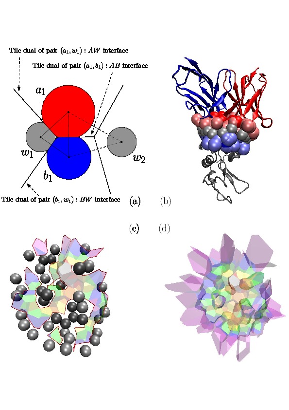 |
Voronoi Interfaces (a) 2D illustration (b c d) Illustration for an IG-Ag complex, whose interaction is mediated by water molecules. |
(a) The Voronoi diagram of four balls (one red particle, one blue particle, two gray water molecules is shown in solid lines). Each ball has been clipped to its Voronoi region, defining its Voronoi restriction . The 


The main specification for
Input. An input PDB file and a specification of the partners (PDB chains).
Main options.
Main output.
Optional output.
Comments.
Bicolor and mediated interfaces come with a number of built-in geometric and topological statistics, which are provided per connected components — see [51] for details:
Tricolor interfaces also have specific built-in statistics:
Assuming that we run intervor over a number of binary complexes, one would want to know statistics about the number of interface particles, or the interface surface area across the complexes. The following python script uses PALSE over the generated xml files to get these statistics:
In a manner analogous to multiple sequence alignments, it is often useful to inspect on the sequence which a.a. are at the interface. This functionality is provided by the script sbl-intervor-ABW-atomic-interface-string.py, which can be called right after intervor itself:
sbl-intervor-ABW-atomic.exe -f data/1vfb.pdb -P AB -P C -d results
sbl-intervor-ABW-atomic-interface-string.py -f 1vfb.pdb -p AB -q C -d results
For example, one obtains the following for chain A – note the three stretches corresponding to the 3 CDRs:
---------------------------N-HNY----------------YY-TT--D----------------------------------FWST-R-----------
In the following, we are concerned with the interface of a complex whose partners have a hierarchical structure.
As an application, we consider the particular case of antibodies whose FAB (fragment antigen-binding) can be decomposed into domains contributed by the heave (H) and light (L) chains respectively.
In the SBL, this case is provided by the program
The case of binary interactions mediated by water molecules easily generalizes to the case where each of the partners has a hierarchical structure i.e. can be partitioned into sub-systems.
Consider e.g. an immunoglobulin whose isotype is IgD or IgE or IgG (the IG involves one monomer of two heavy and two light chains, see e.g. the Wikipedia Antibody or the ImMunoGeneTics information system (IMGT) pages), and assume this IG makes up an IG-Ag complex. Such an IG may be considered in three guises:
Thus, if this IG is involved in an IG-Ag complex, this interaction may be studied at three different levels. As a pre-requisite to do so, we introduce hierarchical decompositions of molecular systems.
To study interfaces, the complex under scrutiny admits a hierarchical decomposition into labels MolecularSystemLabelsTraits, each of them being identified by a label. That is, we assume that the trees encoding these labels correspond to the partners, the mediators, and the extras. Recall that the molecular system associated with a label 
Note that each category of labels (the partners, the mediators and the extras) yields a forest of labels whose leaves are called primitive labels. The forest is possibly reduced to a tree, itself possibly reduced to a singleton.
In the following, we call 

The Voronoi interfaces involving only primitive labels are called primitive interfaces , while all other Voronoi interfaces are called hierarchical interfaces . As illustrated on Fig. Hierarchical interfaces, the two goals are:

Assuming that the partners' forest and the mediators' forest are given, we first compute all the primitive interfaces in three steps, illustrated on Fig. Hierarchical interfaces for the case of an IG-Ag complex:


Note that the interfaces provide information on intra-molecular contacts thanks to the interface 


Hierarchical bicolor interface: 
Hierarchical mediated interface: 
Hierarchical tricolor interface: 
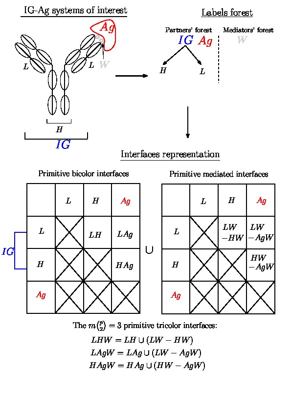 |
Hierarchical interfaces Decomposition of the IG-Ag complex into molecular systems and hierarchical interfaces (Top Left) Schematic representation of an IG-Ag complex with the different labels of the molecular systems involved. (Top Right) Corresponding partners' and mediators' forests. Note that the partners' forest has two trees. (Bottom) Representation of all possible primitive interfaces (bicolor and mediated on the matrix, tricolor under the matrix). |
Input. A PDB file for the IG - Ag complex. We ambition to study the interfaces between the heavy and light chains vs the antigen.
The syntax is almost identical to the one we saw before, except that the heavy and light chains have to be specified separately, e.g. -igL A -igH B -ag C).
Main options.
Main output. The main output files are as follows:
The generated log is identical to that generated by
Optional output.
Comments.
The SBL provides VMD, PyMOL, and Web plugins for sbl-intervor-ABW-atomic.exe. Launch the VMD plugin from the SBL catalog under the Extensions menu, start the PyMOL plugin by running sbl_intervor_ABW_atomic in the PyMOL command line, and open the Web plugin from the SBL web plugins launcher page (served locally via sbl-web-plugins-launcher). All three plugins expose the same GUI and capabilities.
 |
sbl-intervor-ABW-atomic plugin user interface. The user interface for the sbl-intervor-ABW-atomic plugin. The typical workflow is: Step 1: Load a molecular structure from a PDB file. Step 2: Specify the two partners by selecting chains from the structure. Step 3: Set other parameters for computation. Step 4: Choose an output directory (optional, a default is provided). Step 5: Launch the computation. Step 6: Inspect the results in the viewer. Step 7: Review the calculation statistics and interface code string in the GUI. |
The algorithm used in the applications of Space_filling_model_interface are standard ones, which we only briefly sketch in the sequel — see [51] for a detailed treatment.
The classification of contacts between particles relies on the
From a topological standpoint, the bicolor and mediated interfaces are so-called manifold interfaces [132] . In a nutshell, this means that a triangle from the regular triangulation contributes at most two edges to this interface. By the Voronoi - Delaunay duality, this also means that the topological neighborhood of a point located in the relative interior of a Voronoi edge bounding an interface Voronoi facet is either a topological disk or half a topological disk. Note that a tricolor interface may not be a manifold interface.
From an algorithmic standpoint, the computation of primitive interfaces relies on two algorithms:
In particular, bicolor and mediated interfaces are manifold interfaces. See [132] for the details.
The curvature of each connected component of all Voronoi interfaces (hierarchical or primitive, bicolor, mediated or tricolor) is computed twice, one calculation for each partner. First, all the Voronoi edges in the interior of the connected component involving the selected partner are gathered. We orientate the Delaunay edges dual of the Voronoi faces incident to the Voronoi edges such that the particles in the selected partner are the sources of these Delaunay edges. Then, we compute the curvature associated to a Voronoi edge using:
The sum of the curvatures of all the interior Voronoi edges of a connected component defines its curvature, and the sum of the curvature of all connected components of an interface defines the curvature of the interface. Note that an unsigned version of the curvature is also computed (when summing the curvatures of interior Voronoi edges, the absolute value of the curvature is considered).
It is also possible, using the option –bsa, to compute the BSA of each partner at the interface, a task taken care of by the package Buried_surface_area . For versions of intervor using atoms, an XML file is dumped, containing the ids of the atoms (atom id, resid, chain id), as well as the BSA. For versions of intervor using pseudo-atoms, only the BSA is dumped.
The programs of Space_filling_model_interface described above are based upon generic C++ classes, so that additional versions can easily be developed for protein or nucleic acids, both at atomic or coarse-grain resolution.
In order to derive such versions, there are two important ingredients, that are the workflow class, and its traits class.
T_Space_filling_model_interface_traits:
T_Space_filling_model_interface_workflow:
See the following jupyter notebook:
We dissect non-hierarchical and hierarchical Voronoi interfaces in macro-molecular complexes.
In the sequel, we consider the following complexes:
For both, we first compute the non-hierarchical Voronoi interface, which just requires specifying which chains make up the two partner. For 1vfb, we further exploit the decomposition of the IG into its H and L chains, which yields a hierarchical Voronoi interface.
import re  #regular expressions
import sys #misc system
import os
import shutil # python 3 only
import matplotlib.pyplot as plt

odir = "results"
if not os.path.exists(odir): os.system( ("mkdir %s" % odir) )


ifiles = ["data/1vfb.pdb",  "data/2ajf.pdb"]
partners = [("AB", "C"),   ("A", "E")]
def compute_AB_interface(ifile, partners, radius = 0., bsa = False):
    if not os.path.exists(odir): os.system( ("mkdir %s" % odir) )

    exe = shutil.which("sbl-intervor-ABW-atomic.exe")
    if not exe:
        print("Executable sbl-intervor-ABW-atomic.exe not found, exiting")
        return

    cmd = "%s -f %s -P %s -P %s --directory %s --verbose --output-prefix \
          --log --interface-viewer vmd --radius-water %f" \
          % (exe,ifile, partners[0], partners[1],odir, radius)
    if bsa:
        cmd += " --bsa"
    print(("Running %s" % cmd))
    os.system(cmd)

    # list output files
    cmd = "ls %s" % odir
    ofnames = os.popen(cmd).readlines()
    print("\nAll output files:",ofnames)


print("Marker : Calculation Started")
compute_AB_interface(ifiles[0], partners[0], 1.4, bsa = True)
compute_AB_interface(ifiles[1], partners[1], 1.4)


print("Marker : Calculation Ended")
This package offers two sources of visualization:
import matplotlib.pyplot as plt
from PIL import Image


fig, ax = plt.subplots(2, 4, figsize=(15,15))

map(lambda axi: axi.set_xticks([]), ax.ravel())

images_1vfb = ["fig/1vfb-complex.png", "fig/1vfb-interface-atoms.png", "fig/1vfb-voronoi-interface.png", "fig/1vfb-interface-residues-all-atoms.png"]
images_2ajf = ["fig/2ajf-complex.png", "fig/2ajf-interface-atoms.png", "fig/2ajf-voronoi-interface.png",     "fig/2ajf-interface-residues-all-atoms.png"]

print("Top row: antibody-antigen complex")
print("Top row: portion of spike of SARS-COV-2 in complex with its RBD")

for i in range(0,4):
    ax[0, i].set_xticks([]); ax[0, i].set_yticks([])
    ax[0, i].imshow( Image.open(images_1vfb[i]) )

    ax[1, i].set_xticks([]); ax[1, i].set_yticks([])
    ax[1, i].imshow( Image.open(images_2ajf[i]) )

#fig.show()

Bicolor and mediated interfaces come with a number of built-in geometric and topological statistics, which are provided per connected components -- aka binding patches: topology, geometry, biochemistry.
Tricolor interfaces also have specific built-in statistics, in particular topology and shelling order.
Such statistics are easily recovered from the files generated, using PALSE, as we illustrate on a couple of examples. In all generality: just spot the label of interest in the XML file, and get the information with PALSE.
from SBL import PALSE
from PALSE import *

def analyze_with_palse():
    database = PALSE_xml_DB()
    odir = "results"
    #database.load_from_directory(odir)
    database.load_from_directory(odir,".*interfaces.xml")

    # interface AB
    num_atoms_at_AB = database.get_leftmost_data_values_from_database("AB_interface_output/AB_interface_statistics/number_of_particles", int)
    surface_areas_at_AB_with_A = database.get_leftmost_data_values_from_database("AB_interface_output/total_Voronoi_area_with_A", float)
    surface_areas_at_AB_with_B = database.get_leftmost_data_values_from_database("AB_interface_output/total_Voronoi_area_with_B", float)

    print("Num. atoms at the interface AB:",num_atoms_at_AB)
    print("Surface area, interface AB:", surface_areas_at_AB_with_A)
    #PALSE_statistic_handle.hist2d(surface_areas_at_AB, "hist-interface-areas-AB.eps")


    # interface ABW
    num_atoms_at_ABW = database.get_leftmost_data_values_from_database("ABW_interface_output/ABW_interface_statistics/number_of_particles", int)
    print("Num. atoms at the interface ABW:",num_atoms_at_ABW)
    surface_areas_at_ABW_with_A = database.get_leftmost_data_values_from_database("ABW_interface_output/total_Voronoi_area_with_A", float)
    surface_areas_at_ABW_with_B = database.get_leftmost_data_values_from_database("ABW_interface_output/total_Voronoi_area_with_B", float)
    print("Surface area, interface ABW:", surface_areas_at_ABW_with_A)

print("Marker : Calculation Started")
analyze_with_palse()
print("Marker : Calculation Ended")
import os
import subprocess

cmd = "mkdir resi"
os.system(cmd)

cmd = "sbl-intervor-ABW-atomic.exe -f data/2ajf.pdb -P A -P E -d resi"
os.system(cmd)

cmd = ["sbl-intervor-ABW-atomic-interface-string.py", "-f", "data/2ajf.pdb", "-p", "A", "-q", "E", "-d", "resi"]
s=subprocess.check_output(cmd, encoding='UTF-8')
print(s)
def compute_AB_hierchical_interface():


    exe = shutil.which("sbl-intervor-IGAgW-atomic.exe")
    if not exe:
        print("Executable sbl-intervor-IGAgW-atomic.exe not found, exiting")
        return


    ifile = "data/1vfb.pdb"
    odir = "results-hierarchical"

    if not os.path.exists(odir): os.system( ("mkdir %s" % odir) )

    cmd = "%s -f %s --igL A --igH B --ag C  --directory %s --verbose --output-prefix --log --interface-viewer vmd" % (exe,ifile,odir)
    os.system(cmd)
    # list output files

    cmd = "ls %s" % odir
    ofnames = os.popen(cmd).readlines()
    print("\nAll output files:",ofnames)

print("Marker : Calculation Started")
compute_AB_hierchical_interface()
print("Marker : Calculation Ended")
Under VMD, we can now visualize in turn (i) the whole IG-Ag interface, (ii) the interafce between the heavy chain and the antigen, (iii) the interface between the light chain and the antigen, and (iv) the interface between the H and L chains.