Structural Bioinformatics Library
Template C++ / Python API for developping structural bioinformatics applications.
User Manual

Authors: F. Cazals and T. Dreyfus and C. Robert and A. Roth

Landscape_explorer

Goals

In this package, we consider the problem of sampling a landscape, that is a height function defined as the real valued multivariate function. In biophysics, we notice, though, that this function typically codes the potential energy of a molecular system, so that the landscape is the potential energy landscape (PEL).

The algorithms presented fall in the realm of Monte Carlo based methods, in a broad sense. The precise meaning of sampling shall depend on the specific algorithms presented, as one may want in particular to:

  • Locate the low lying local minima of the function, with potentially a focus on the global minimum.

  • Generate conformation ensembles meeting specific properties. Typically, speaking of biomolecular systems, one may wish the conformations generated to comply with $\text{\boltz}$'s law.

We actually provide a generic framework to develop such algorithms, providing instantiations for classical algorithms as well as algorithms developed recently.
Of particular interest in the sequel are the following three algorithms:

  • $\text{\algoBH}$: the basin hopping algorithm, which performs a random walk in the space of local minima [118] , [172] .

  • $\text{\algoTRRT}$: the rapidly exploring random trees algorithm, which favors the exploration of yet unexplored space based upon the Voronoi bias [99] .

  • $\text{\algoHY}$: a hybrid algorithm mixing the merits of $\text{\algoBH}$ and $\text{\algoTRRT}$ [153] .

Practically, our main focus is on landscapes encoding the potential energy of a molecular system. Yet, our algorithms also handle the case of a multivariate real-valued function void of biophysical meaning. The ability to handle such diverse cases owes to a generic framework. We illustrate it by providing explorer in three settings:

  • For a protein model known as BLN69, defined over a configuration space of dimension 3x69=207, see section BLN69,

  • For small peptides such as pentalanine using the Amber force field, defined over a configuration space of variable dimension (3x53=159 for pentalanine),

  • For real valued function of several variables, namely the 2D Rastrigin function and the trigonometric terrain presented in section Example Landscapes defined from mathematical functions.

Needless to stress that these are simple examples, and that instantiations of our exploration algorithms are easily derived by instantiating our generic classes.

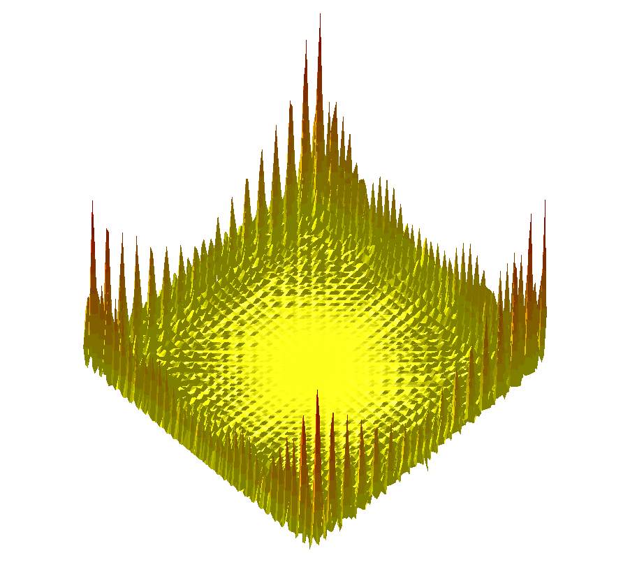
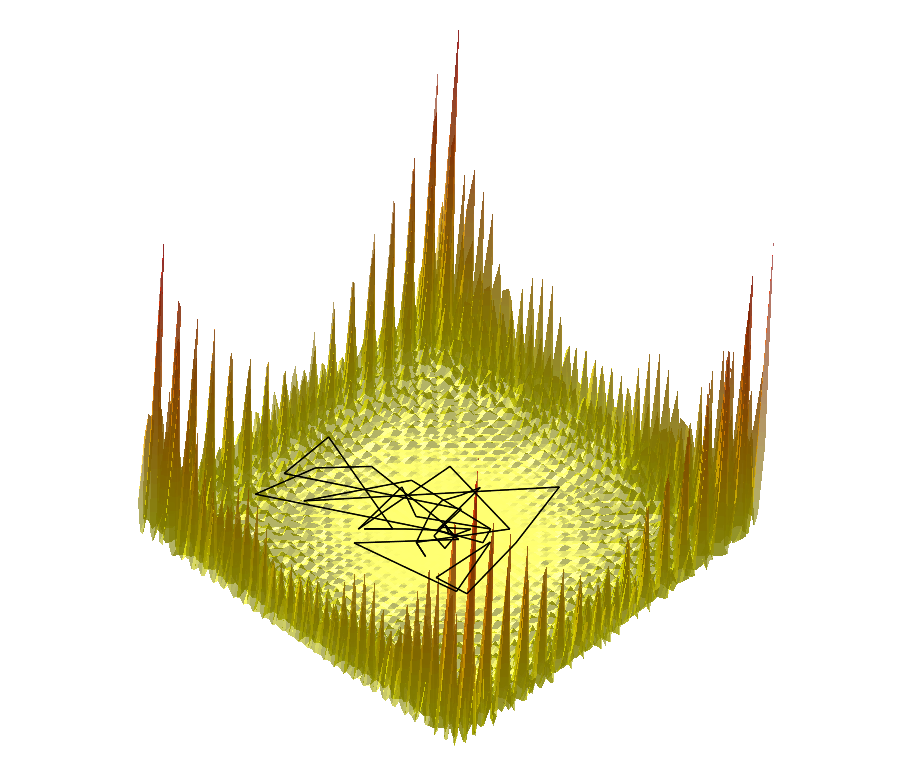
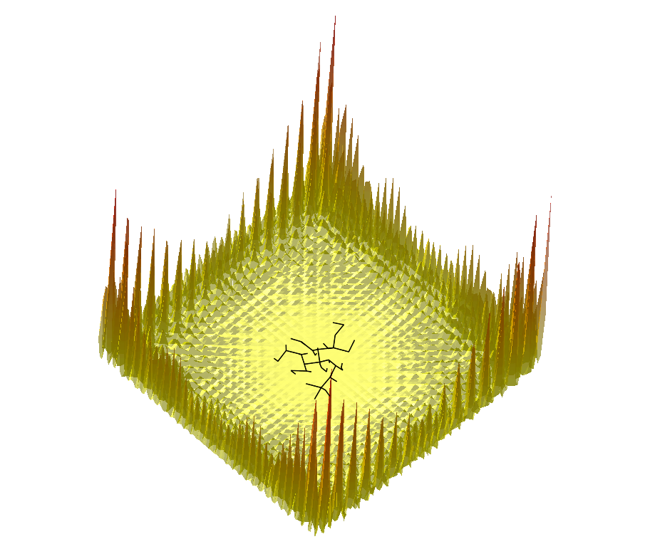
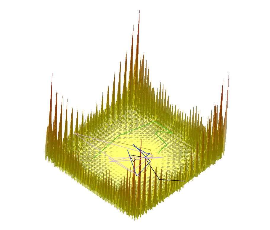
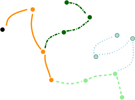
Comparing the explorations on the trigonometric terrain

Top.Trigonometric terrain to be explored : $f(x,y)=(x\sin(20y)+y\sin(20x))^2\cosh(\sin(10x)x)+(x\cos(10y)-y\sin(10x))^2\cosh(\cos(20y)y)$

Bottom. From Left to Right : Basins Hopping, TRRT and Hybrid. 50 minima (samples for TRRT) were generated. For TRRT, the initial displace delta was 0.5, while for Basins Hopping and Hybrid, it was 0.0001. For the Hybrid algorithm, Basins Hopping is used 10 times, then TRRT is used once : the consecutive minima generated by Basins Hopping are linked with rays of the same color.

A generic / template algorithm

We first introduce a generic algorithm, thanks to which we shall instantiate all our algorithms.

Generic algorithm. A generic template (Algorithm alg-landexp-generic) describes the three aforementioned algorithms, and a number of variants. In addition to a stop condition (stating e.g. whether the number of conformations desired has been reached), this template consists of six main steps, namely:

  • $\text{\selectConf}$: a function selecting the conformation to be extended, denoted $p_n$.

  • $\text{\extendConf}$: a function generating a new conformation, denoted $p_e$, from the conformation just selected. As we shall see below, an extension is an operation consisting of one or several calls to a move set operation (see definition bln-movesets).

  • $\text{\acceptConf}$: Test of the Metropolis type, stating whether the new conformation is accepted or not.

  • $\text{\recordConf}$: A function incorporating the sample just accepted into a data structure representing the growing set of configurations.

  • $\text{\updateMoveSetParams}$: adaptation of the move set parameters, used by the extension algorithm. (Intuitively, the extension should not call too many move steps.)

  • $\text{\updateAcceptParams}$: update of the parameters governing the acceptance test—in particular temperature adaption. Intuitively, the acceptance ratio should not fall below a prescribed value.

\begin{algorithm} \begin{algorithmic} \REQUIRE{$\energyP{p}$: potential energy function of a given conformation $p$} \REQUIRE{Parameters governing the exploration, typically the temperature $T$ and the step size $\delta$} \REQUIRE{$P:$ data structure hosting the conformations harvested} \STATE{} \STATE{Initialize the set $P$ with one conformation} \WHILE{\stopCond = False} \STATE{$p_{n} \leftarrow \selectConf{P}$} \STATE{} \STATE{//Extend, i.e. iteratively generate a new conformation until success} \STATE{//and possibly update the generation parameters} \STATE{//via a function call to $\updateMoveSetParams$} \STATE{$p_{e}\leftarrow \extendConf{p_{n}}$} \STATE{} \IF{$\acceptConf{p_{n}, p_{e}}$} \STATE{$\recordConf{p_e, P}$} \ENDIF \STATE{$\updateAcceptParams$} \ENDWHILE \end{algorithmic} \caption{{\bf Algorithm \gensampler: a generic sampling algorithm for potential energy landscapes.}} \end{algorithm}

Parameters of the algorithm. By parameters of an algorithm, we refer to the variables and constants which shape its behavior. We distinguish four types of parameters (Fig. fig-landexp-explo-params):

  • Exploration variables: the core variables governing the exploration. The typical such variables are the temperature $T$ and the step size $\delta$ – the step size is used by the move set. These variables are generally global, but may also be made local so as to account for specific features of the landscape. For example, the values of $\delta$ and $T$ may be locally adapted to the topography of the landscape. When necessary, in presenting the algos, we distinguish:

    • Exploration variable
    • Acceptance variables

  • Tuning constants: multiplicative values used to evolve the exploration variables.

  • Control constants: the constants controlling how exploration variables are evolved. The typical constants are:

    • Exploration variables: target probability for the success of an extension.

    • Acceptance variables: the target probability for the acceptance of a sample, number of rejections of the acceptance test before tuning the parameters.

  • Identity constants: constants used to decide whether two conformations have the same energy (threshold $\boundEner$), or to decide whether two conformations are identical (distance threshold $\boundDist$, say on the $\lrmsd$).

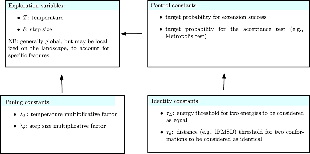
Exploration parameters
Parameters i.e. variables and constants used by the algorithms.

Details for $\text{\selectConf}$. The function $\text{\selectConf}$, which selects the conformation to be extended, may require a distance threshold, denoted $\boundDist$, and an energy threshold, denoted $\boundEner$ (see e.g. $\text{\algoTRRT}$). When the selection is performed amidst a large database of conformations, the execution speed may be improved using data structures providing fast retrieval of nearest neighbors. This is in particular the case if the $\lrmsd$ is used as a distance. In any case, to initialize the algorithm, a database (possibly reducing to a single conformation0 of samples to select conformations from must be passed.

The main options are: –distance-epsilon string: distance threshold below which conformations are identical
–height-epsilon string: threshold below which energies are identical
–init-sample string: a set of conformations to initialize the selection process


Details for $\text{\extendConf}$. A move set is a unitary operation thanks to which a new conformation is generated from a given conformation, typically at a predefined distance called the step size denoted $\delta$. Three classical move sets are the so-called global moveset, interpolation moveset, and atomic moveset, as detailed in section bln-movesets.

To perform an extension, see function $\text{\extendConf}$ above, it might be necessary to iterate the generation step using the move set until some conditions are fulfilled, see algorithms $\text{\algoBH}$ and $\text{\algoTRRT}$ below.

In selected cases, the extension requires minimizing the potential energy, aka quenching. While computing the gradient can be done using symbolic differentiation tools such as Maple or Mathematica, it can also be computed by automatic differentiation of the C/C++ code, using e.g. the Tapenade software. This solution is flexible as any energy function can easily be differentiated.
Note also that alternatives to the full gradient may be used, such as a truncated gradient (one may selected the largest partial derivatives), a randomized one-dimensional gradient (one partial derivative chosen at random), etc.


Because the extension is in general an expensive operations, an adaptation mechanism for the parameters governing the move set is called for, whence the function $\text{\updateMoveSetParams}$.

The main options are: –moveset-mode string: setting the move set
–displace-delta string: setting the step size for the move set
–adaptive-displace-delta string:
setting the number of consecutive fails to extend parameters should be updated
–target-proba-displace-delta string: setting the target probability of updating the step size each time the number of consecutive fails reaches that target number.


Details for $\text{\acceptConf}$. The prototypical acceptance test is the Metropolis criterion, which merely requires a temperature $T$ [112] .

The main options are:
–temperature string: setting the initial temperature used in the Metropolis test
–Boltzmann-constant float(= multiplicative constant used in the exponant of the metropolis criterion (default is 1): i.e no multiplicative factor)


Details for $\text{\updateAcceptParams}$. After the acceptance test is performed, the temperature can be updated through a multiplicative factor $\lambda_T$.

Yet, several default tuning modes are offered:

  • the default method consists on decreasing the temperature each time a sample is accepted, and increasing the temperature after a number of consecutive failures.

  • the probability method attempts to reach a given target acceptance ratio for the acceptance test. In this mode, every $N$ acceptance tests, the acceptance ratio observed since the beginning of the run is computed. A temperature update is triggered if this ratio is less than the target.

  • the energy-range method used energy range of the conformations discovered so far for udpating the temperature [112]
The main options are: –temperature-tuning-mode string: setting the temperature tuning mode (default, probability, energy-range)
–lambda-T string: setting the multiplicative factor to tune the temperature
–temperature-max-reject string: number of consecutive rejections triggering an increase of the temperature
–target-proba-acceptance string: target acceptance ratio for the Metropolis test
–nb-tests-tuning string: frequency to check whether the acceptance ratio is above or below the target probability


Details for $\text{\recordConf}$.

In recording conformations, we face two cases which are detailed below:

  • Conformations are stored into a plain vector which is later dumped onto the disk. The linear nature of the vector container does not allow efficient filtering to avoid duplicates i.e. conformations discovered several times. Avoiding duplicates is of particular interest if conformations are local minima.
  • Conformations are stored in data structures providing efficient ways to identify and filter out duplicates. Such data structures may focus on the energy or the coordinates/distances between conformtions.

Without filtering data structure: the case of $\text{\algoBH}$. If no filtering is carried out during the execution, duplicates are easily sorted out upon termination with a script, e.g.:

If one wants to avoid redundancy while using $\text{\algoBH}$, it can be easily done through a bash script, as follows :
rm -f $1_uniq.txt; touch $1_uniq.txt;
rm -f $1_energies_uniq.txt; touch $1_energies_uniq.txt;
zero=0
i=1
while read p; do
    count=$(grep -c "$p" "$1_uniq.txt")   
    if [ "$count" -eq "$zero" ]; then
        echo "$p" >> "$1_uniq.txt"
        sed "${i}q;d" "$1_energies.txt" >> "$1_energies_uniq.txt"
    fi
    ((i++))
done < $1.txt
Indeed, this does not guarantee anymore the number of different minima / samples that have been visited.


With filtering data structure: the case of $\text{\algoTRRT}$ and $\text{\algoHY}$.

As mentioned above, filtering consists in identifying duplicates, at a sub-linear cost with respect to the conformations already identified. We distinguish filtering on the energy and on distances.

Filtering on energy commonly consists of checking that the energy of a newly found conformation differs by an amount $\boundEner$ from those collected so far. To be performed in logarithmic time, this check requires a dictionary storing conformations and their energies.

Filtering on energies is in general not sufficient though, since the set, in conformational space, of conformations having a prescribed energy is generically a $d-1$ manifold, with $d$ the dimension of the conformational space.

To filter on distances (e.g., using the least root-mean-square deviation, $\lrmsd$), several alternatives are possible. One approach consists of assigning an energy (bin) to all local minima having energy in this bin. Upon discovering a novel minimum, it is then sufficient to compute distances from local minima stored with that energy, retaining the new candidate provided that its nearest neighbor is at least at some predefined distance $\boundDist$. A second approach consists of using data structures supporting (approximate) nearest neighbor queries [155] . For queries under the $\lrmsd$ distance in particular, one may use metric trees ~[178] or generalizations such as proximity forests~[139] . This strategy also allows guaranteeing a minimum distance $\boundDist$ between any two conformations.

Details for $\text{\stopCond}$. Four different stop criteria are currently offered:

  • the number of samples criterion : the algorithm stops when a number of registered conformations is reached.

  • the landmarks criterion: the algorithm stops once given specified landmarks have been visited—up to a distance criterion.

  • the quenched to landmarks criterion: each sample is quenched, and the algorithm halts when the local minima specified have been visited—up to a distance criterion.

  • the connected criterion : the algorithm stops once the graph represented the exploration is connected. Note that $\text{\algoBH}$, the graph is a path and is always connected. In fact, this option is useful for $\text{\algoTRRT}$ or $\text{\algoHY}$, when several conformations are used to initialize the algorithm.
The main options are: –stop-mode string: stop mode out of the four offered options (nb-samples, landmarks, quenched-to-landmarks, connected)
–nb-samples string: stop when reaching a predefined number of samples
–landmarks string: stop when all the specified landmarks have been visited (up to a distance threshold)


Using Basin Hopping (BH)

Pre-requisites

Instantiation for $\text{\algoBH}$. We now present the functions used by $\text{\algoBH}$, explaining in particular how the parameters of the algorithm (temperature $T$, step size $\delta$) are adapted:

  • $\text{\selectConf}$: for $\text{\algoBH}$, this function simply returns the last local minimum generated.

  • $\text{\extendConf}$: a function applying a move set to the conformation to be extended, then quenching it. This process is iterated until a novel local minimum is discovered–equivalently, the conformation generated must leave the catchment basin of the local minimum being extended.

  • $\text{\acceptConf}$: the Metropolis Transition test.

  • $\text{\recordConf}$: Adds the local minimum just accepted to the path of local minima being generated.

  • $\text{\updateMoveSetParams}$: In the $\text{\algoBH}$ used here, the stepsize $\delta$ is adapted so as to reach a target probability – representing the fraction of extended samples escaping the current basin. The update is performed at a predetermined frequency with respect to the number of extension attempts.

  • $\text{\updateAcceptParams}$: Temperature adaptation is performed to achieve a target fraction of accepted samples. If the target value is surpassed, the temperature is decreased, otherwise it is increased after a fixed number of iterations.

\begin{algorithm} \begin{algorithmic} \REQUIRE{$current\_proba$: fraction of so far accepted points\\ $target\_proba$: desired value for $current\_proba$\\ $nb\_accepts$: number of accepted points\\ $nb\_attempts$: number of attempts for the previous\\ $nb\_temp\_check$: frequency at which the condition on $target\_proba$ is checked} \IF{$nb\_attempts \% nb\_temp\_check == 0$} \STATE{$current\_proba \leftarrow nb\_accepts / nb\_attempts$} \IF{$current\_proba > target\_proba$} \STATE{$T \leftarrow T * \lambda_T$} \ELSE \STATE{$T \leftarrow T / \lambda_T$} \ENDIF \ENDIF \end{algorithmic} \caption{{\bf Temperature adaptation for \algoBH.} The temperature $T$ is adapted in \algoBH (and also \algoHY) as to tend towards a target probability, representing the fraction of accepted samples desired.} \end{algorithm}

The basin hopping algorithm
The algorithm performs a walk in the space of local minima. Upon generating a new conformation by applying a move set to a local minimum $m_i$, this conformation is minimized by following the negative gradient of the energy, yielding a local minimum $m_{i+1}$.

Main specifications

BH may be used to explore any model (mathematical function, toy protein model BLN, regular atomic model, etc). Since every such model yields a different executable, this executable is referred to as sbl-landexp-BH-NAME-OF-MODEL.exe in the sequel.

The Jupyter notebook provided in this user manual uses several such executables.

Main options.

The main options of the program sbl-landexp-BH-NAME-OF-MODEL.exe are:
–init-sample string: plain text file listing at least one conformation for initaliwing the explorer
–moveset-mode: moveset method (global, interpolation)
–adaptive-displace-delta: number of steps after what the algorithm attempts to adapt
–temperature-tuning-mode: updating method after the acceptance test (default, probability or energy-range
–nb-samples int: number of samples to record before stopping the algorithm


Input.

  • (Point_d format) Conformations: list of samples / conformations to get started. Note that for BH, the algorithms starts from the last sample.

Main output.

  • (txt format, suffix log.txt) Main log file, containing high level information on the run.
  • (Point_d format, suffix samples.txt) Samples, geometry: samples generated, one sample per line.
  • (txt format, suffix samples_energies.txt) Samples, energies: energy of each sample in the previous file.
  • (Point_d format, suffix minima.txt) Minima, geometry: minima found, one minimum per line.
  • (PDB format, suffix minimumINTEGER.vmd) Minima, PDB: one PDB file for each local minimum.
  • (txt format, suffix minima_energies.txt) Minima, energies: energy of each local minimum.

Optional output.

Comments.

Using Transition based Rapidly Exploring Random Trees (T-RRT)

Pre-requisites

Instantiation for $\text{\algoTRRT}$. The method generates a tree spanning the conformational space. Following [99] , the steps are:

  • $\text{\selectConf}$: this function generates uniformly at random a configuration $p_r$ in the conformational space, and returns the local minimum $p_n$ nearest to it. This strategy promotes samples with large Voronoi regions– intuitively corresponding to regions with low sampling density– as a sample is selected with a probability proportional to the volume of its Voronoi region~[110] . We call this property the Voronoi bias (selection) rule hereafter.

  • $\text{\extendConf}$: the new conformation $p_e$ is obtained by linearly interpolating between $p_r$ and $p_n$, at a predefined distance $\delta$ from $p_n$.. Note that by the convexity of Voronoi regions, the new sample remains within the Voronoi cell of $p_n$. It is also possible to iteratively generate a new conformation until the new conformation lies in the current Voronoi cell, i.e. in the Voronoi cell of the sample chosen for extension – as one may indeed generate a new conformation outside this Voronoi cell.

  • $\text{\acceptConf}$: Metropolis test as for $\text{\algoBH}$. (See also remark rmk-energy-range .)

  • $\text{\recordConf}$: the accepted sample is used to add the edge $(p_n, p_e)$ to the random tree grown.

  • $\text{\updateMoveSetParams}$: in $\text{\algoTRRT}$, the step size is constant.

    NB: the previous is sufficient when using an interpolation scheme to extend the point selected. (If the euclidean distance is used, by convexity of Voronoi regions, any point on the line-segment $[p_n,p_i]$ lies in the Voronoi cell of $p_n$.) The situation differs in using a move set, since the point generated might be located outside the Voronoi region targeted. In that case, the extension requires generating samples until a point in the Voronoi region targeted has been found. This may require a step size adaptation—a situation analogous to that faced in $\text{\algoBH}$.

  • $\text{\updateAcceptParams}$: upon accepting a sample with increasing energy, the temperature is tuned using the range of energies of samples already inserted into the tree (supplemental algorithm alg-adaptTd-algoBH and [69]).

    temperature adaptation taking into account the maximal energy variation of the conformational ensemble generated

Practically, the Voronoi diagram for the set of samples cannot be built, as its complexity is exponential in the dimension. The Voronoi bias rule thus exploits the structure of the Voronoi diagram implicitly, via nearest neighbor searches.


In [69], [68] , the range of energies associated with samples discovered is maintained. This range is used to tune the temperature as follows (algorithm alg-adaptTd-algoTRRT):
  • If we transition to a point at a lower energy, the temperature is not changed;
  • Otherwise, the transition is subject to the Metropolis criterion:

    \begin{align} T \text{ decreased upon acceptance: } & T /= 2^{(E(p_n)-E(p_e))/energyRange*0.1}\\ T \text{ increased upon rejection: } & T *= 2^c, \text{ with } c \text{ fixed.} \end{align}


\begin{algorithm} \begin{algorithmic} \REQUIRE{$E_{new}$: energy of the point to be inserted\\ $E_{old}$: energy of the currently processed point\\ $lambda$: preset parameter\\ $C$: the current conformational ensemble\\ $energyRange$: the current maximal energy variation of the conformational ensemble} \IF{$ E_{new} > E_{old} $} \IF{$p_{new}$ is accepted} \STATE{$T \leftarrow T / 2^{(E_{new}-E_{old})/0.1 * energyRange(C)}$} \ELSE \STATE{$T \leftarrow T * 2^{\lambda}$} \ENDIF \ENDIF \end{algorithmic} \caption{{\bf Temperature adaptation for \algoTRRT.} In \algoTRRT, the adaptation takes into account the maximal energy variation of the present conformational ensemble, as in \cite devaurs2013multi .} \end{algorithm}

Main specifications

TRRT may be used to explore any model (mathematical function, toy protein model BLN, regular atomic model, etc). Since every such model yields a different executable, this executable is referred to as sbl-landexp-TRRT-NAME-OF-MODEL.exe in the sequel.

The Jupyter notebook provided in this user manual uses several such executables.

Main options.

The main options of the program sbl-landexp-TRRT-NAME-OF-MODEL.exe are:
–init-sample string: plain text file listing at least one conformation for initaliwing the explorer
–moveset-mode: moveset method (atomic, global interpolation)
–nb-samples int: number of samples to record before stopping the algorithm


Input.

  • (Point_d format, suffix txt) Samples: list of samples / conformations to get started. Note that for TRRT, these samples are used to initialize the spatial search data structure, from which the next sample extended is chosen – using the Voronoi bias.

Main output.

Identical to that of Basin-hopping, see above.

Optional output. Comments.

Using a hybrid algorithm (Hybrid) combining BH and T-RRT

Pre-requisites

Intuitively, our hybrid algorithm may be seen as a variant of $\text{\algoBH}$ in which, instead of systematically extending the local minimum just found, the Voronoi bias rule from $\text{\algoTRRT}$ is used every $b ( > 1)$ $\text{\algoBH}$ steps, in order to select the local minimum to be extended. In the following, the parameter $b$ is called the switch parameter. Similarly to $\text{\algoTRRT}$, the algorithm generates a tree connecting local minima. In $\text{\algoHY}$, however, this tree can be partitioned into threads, each thread consisting of local minima generated by a contiguous sequence of extensions and quenches of $\text{\algoBH}$ (Fig. fig-landexp-algoHY).

More precisely, $\text{\algoHY}$ uses the following five functions to instantiate the generic algorithm~alg-landexp-generic :

  • $\text{\selectConf}$: once every $b$ steps, the Voronoi bias is used to select the local minimum to be extended. For the remaining steps, the sample to be extended is the last local minimum generated.

  • $\text{\extendConf}$: the extension strategy is identical to that used in $\text{\algoBH}$. (NB: this departs from $\text{\algoTRRT}$ in that here a move set is used, as opposed to an interpolation scheme.)

  • $\text{\acceptConf}$: the acceptance test is identical to that used in $\text{\algoBH}$.

  • $\text{\recordConf}$: the record step is identical to that used in $\text{\algoBH}$.

  • $\text{\updateMoveSetParams}$: upon starting a new thread, i.e. upon selecting a sample to extend using the Voronoi bias rule, the step size is re-initialized.

  • $\text{\updateAcceptParams}$: similar to $\text{\updateMoveSetParams}$ – temperature is re-initialized.

The following important remarks are in order:

  • The switch parameter $b$ can be optimized to best exploit features of a given PEL [153] .

  • For the extension strategy, using a move set (rather than the interpolation in $\text{\algoTRRT}$) provides much more flexibility. This turns out to be critical to focus the exploration on low energy regions.

  • In the parameter update step, resetting the parameters upon starting a new thread is also critical, as this allows locally adapting the parameters to the landscape. Because $\text{\algoTRRT}$ explores very diverse regions of the PEL thanks to the Voronoi bias rule, failure to reinitialize may result in using inappropriate parameter values. We note in passing that an alternative to the reset was tested in which each local minimum was stored with the parameters it was discovered with–see comments on the memory mechanism in the Results section.

  • A key operation in $\text{\algoTRRT}$ is that of locating the nearest neighbor $p_n$ of the random sample $p_r$, as $p_n$ is the node undergoing the extension. To facilitate this step, we use data structures designed for searching nearest neighbors in metric spaces, namely random forests of metric trees [178], [139] . Practically, since the move set is implemented in Cartesian coordinates, the metric used for nearest neighbor queries is the RMSD.

The $\text{\algoHY}$ algorithm
$\text{\algoHY}$ consists of interleaving calls to $\text{\algoTRRT}$ and $\text{\algoBH}$. In this cartoon, starting from the initial configuration (black dot), one step of $\text{\algoTRRT}$ is performed after every three steps of $\text{\algoBH}$ (i.e., $b=3$). The local minima generated by a contiguous sequence of $\text{\algoBH}$ extensions and quenches are represented with the same color. Each such set of local minima is also called a thread. Thus, in this example, $\text{\algoHY}$ has generated four threads of size three.

Main specifications

Hybrid may be used to explore any model (mathematical function, toy protein model BLN, regular atomic model, etc). Since every such model yields a different executable, this executable is referred to as sbl-landexp-hybrid-NAME-OF-MODEL.exe in the sequel.

The Jupyter notebook provided in this user manual uses several such executables.

Main options.

The main options of the program sbl-landexp-hybrid-BH-TRRT-*.exe are:
–init-sample string: plain text file listing at least one conformation for initalizing the explorer
–moveset-mode: moveset method (atomic, global or interpolation)
–nb-main-selector int: number of consecutive steps using the main selector before switching to the hybrid selector
–nb-hybrid-selector = 1 int: number of consecutive steps using the hybrid selector before switching to the main selector
–nb-samples int: number of samples to record before stopping the algorithm
–cs-pdb-files string: for amber : pdb file for loading the covalent structure of the peptide
–ff-parameters string: for amber : force fields parameters file name
–ff-length-in-nanometer bool: input parameters are in nanometers rather than angstroms
–ff-length-in-kilojoule string: input parameters are in kilojoules rather than kilocalories
–ff-length-in-coulomb string: input parameters are in coulomb rather than elementary charge


Input.

  • (Point_d format, suffix txt) Samples: list of samples / conformations to get started. These samples are used to initialize the spatial search data structure, from which the next sample extended is chosen – using the Voronoi bias.

In dealing with atomic molecular models in general and proteins in particular, the following are also needed:

  • (PDB format) Topology file:
    the PDB file implicitly encodes the covalent structure.

Main output. Whatever the system, the output files are as described previously:

Identical to that of Basin-hopping and TRRT, see above.

Optional output.

Comments.

Algorithms and Methods

All algorithms presented in this package follow the generic template of fig. alg-landexp-generic.

They use different ingredients, including (i) calculation of the potential energy (see packages Molecular_covalent_structure, Molecular_potential_energy) (ii) evaluation of the gradient of a real-value function (see package Real_value_function_minimizer), and (iii) spatial data structures for nearest neighbor searches (see package Spatial_search).

Note that the computation of the gradient is only semi-automatized, as mentioned in Remark. 1 of section A generic / template algorithm . In particular, the user should provide its own implementation of the gradient of the energy function, whatever is the source. An option is to use an automatic differentiation tool such as Tapenade to generate this gradient.

External Dependencies

In addition to the usual external libraries used in the SBL (CGAL, Boost, Eigen), this package is using two other external libraries :

  • LBFGS++ (mandatory) : used for the gradient calculation during the minimization step.
  • rapidxml (mandatory) : used for loading force field parameters stored in FFXML files.

Programmer's Workflow

The programs of Landscape_explorer described above are based upon generic C++ classes, so that additional versions can easily be developed.

In order to derive other versions, there are two important ingredients, that are the workflow class, and its traits class.

The Traits Class

T_Landscape_explorer_traits:

The Workflow Class

T_Landscape_explorer_workflow:

Jupyter demo

See the following jupyter notebook:

  • Jupyter notebook file
  • Landscape_explorer

    Landscape_explorer

    The exploration of an energy landscape may focus on different features:

    * the extent explored
    * the identification of (deep) local minima
    * the identification of saddle points / transition points
    

    In the following, we illustrate three different methods, which in a nutshell may be characterized by:

    * Basin-hopping: focus on local minima -- see below
    * Rapidly exploring random trees: focus on the extent visited and transition states
    * Hybrid: mix between BH and T-RRT
    

    Results are presented for the following systems:

    * a complex trigonometric function defined 
    * BLN69, a toy protein model, whose conformation requires 3x69=207 Cartesian coordinates
    * Penta-alanine, aka Ala5

    We first define some useful functions

    In [1]:
    import re
    import math
    import numpy as np
    import matplotlib.pyplot as plt
    
    from scipy.cluster.hierarchy import dendrogram, linkage
    from scipy.spatial.distance import squareform
    
    from scipy.cluster.hierarchy import dendrogram, linkage
    from matplotlib import pyplot as plt
    
    # A Function to be used later to retrieve specific output files
    def find_file_in_output_directory(str, odir):
        cmd = "find %s -name *%s" % (odir,str)
        return os.popen(cmd).readlines()[0].rstrip()


    def plot_dendogram_of_conformations(distances):
        # read the n(n-1)/2 distances and compute n
        lines = open(distances, "r").readlines()
        s = len(lines)
        n = int((1+math.sqrt(1+8*s))/2)
    
        # load distances into np array
        mat = np.zeros((n,n))
        for line in lines:
            aux = re.split("\s", line.rstrip())
            mat[int(aux[0]), int(aux[1])] = float(aux[2])
            mat[int(aux[1]), int(aux[0])] = float(aux[2])
    
        # plot dendogram
        dists = squareform(mat)
        linkage_matrix = linkage(dists, "single")
        dendrogram(linkage_matrix, labels= list(range(0,n+1)))
        plt.title("Conformations: dendogram based on lrmsd")
        plt.show()
    

    Example : trigonometric terrain

    Let us first visualize the graph of the trigonometric function studied:

    $ f(x,y)=(x\sin(20y)+y\sin(20x))^2\cosh(\sin(10x)x)+(x\cos(10y)-y\sin(10x))^2\cosh(\cos(20y)y)$

    In [2]:
    import matplotlib.pyplot as plt
    from PIL import Image
    
    fig, ax = plt.subplots(1, 3, figsize=(100,100))
    images = ["fig/bh-trigo-50.png", "fig/trrt-trigo-50.png", "fig/hybrid-trigo-50.png"]
    
    for i in range(0,3):       
        ax[i].set_xticks([]); ax[i].set_yticks([])
        ax[i].imshow( Image.open(images[i]) )
    print("Displayed")    
    
    Displayed
    

    The options of the runTrigo method in the next cell are:

    • algorithm: algorithm to use (BH, TRRT, hybrid)
    • initSample: plain text file listing at least one conformation for initaliwing the explorer
    • movesetMode: moveset method (global, interpolation)
    • delta: number of steps after what the algorithm attempts to adapt
    • temperature: initial temperature used in the acceptance test
    • tempMode: updating method after the acceptance test (default, probability or energy-range
    • nbSamples: number of samples to record before stopping the algorithm
    In [3]:
    import re  #regular expressions
    import sys #misc system
    import os
    import pdb
    import shutil # python 3 only
    
    def runTrigo(algorithm, initSample = None, movesetMode = "global", delta = 5, temperature = 2., \
                 tempMode = "probability", nbSamples = 10):
    
        odir = "tmp-results-trigo-%s" % algorithm 
        if os.path.exists(odir):
            os.system("rm -rf %s" % odir)
        os.system( ("mkdir %s" % odir) )
        
        program = None
        if algorithm == "BH":
            program = "sbl-landexp-BH-trigo-terrain.exe"
        elif algorithm == "TRRT":
            program = "sbl-landexp-TRRT-trigo-terrain.exe"
        elif algorithm == "hybrid":
            program = "sbl-landexp-hybrid-BH-TRRT-trigo-terrain.exe"
        # check executable exists and is visible
        exe = shutil.which(program)
        if not exe:
            sys.exit("Executable %s not found, exiting" % program)
        
        print(("Using executable %s\n" % exe))
        if initSample:
            cmd = "%s -v1 -l --init-sample=%s \
                    --moveset-mode=%s --temperature=%f \
                    --temperature-tuning-mode=%s --nb-samples=%d --directory=%s" \
                    % (program, initSample, movesetMode, temperature, tempMode, nbSamples, odir)
        else:
            cmd = "%s -v1 -l --moveset-mode=%s \
                    --temperature=%f --temperature-tuning-mode=%s \
                    --nb-samples=%d --directory=%s" \
                    % (program, movesetMode, temperature, tempMode, nbSamples, odir)
        if algorithm != "TRRT":
            cmd += " --adaptive-displace-delta=%d" % delta
        print(("Executing %s\n" % cmd)) 
        os.system(cmd)
            
        cmd = "ls %s" % odir
        ofnames = os.popen(cmd).readlines()
        print(("All output files in %s:" % odir),ofnames)
        
    
    In [4]:
    print("Marker : Calculation Started")
    runTrigo("BH", initSample = "data/origin-2D.txt")
    #runTrigo("TRRT", initSample = "data/origin-2D.txt")
    #runTrigo("hybrid", initSample = "data/origin-2D.txt")
    print("Marker : Calculation Ended")
    
    Marker : Calculation Started
    Using executable /user/fcazals/home/projects/proj-soft/sbl-install/bin/sbl-landexp-BH-trigo-terrain.exe
    
    Executing sbl-landexp-BH-trigo-terrain.exe -v1 -l --init-sample=data/origin-2D.txt                 --moveset-mode=global --temperature=2.000000                 --temperature-tuning-mode=probability --nb-samples=10 --directory=tmp-results-trigo-BH --adaptive-displace-delta=5
    
    All output files in tmp-results-trigo-BH: ['sbl-landexp-BH-trigo-terrain__log.txt\n', 'sbl-landexp-BH-trigo-terrain__minima_energies.txt\n', 'sbl-landexp-BH-trigo-terrain__minima.txt\n', 'sbl-landexp-BH-trigo-terrain__samples_energies.txt\n', 'sbl-landexp-BH-trigo-terrain__samples.txt\n']
    Marker : Calculation Ended
    

    The files containing the samples, minima, and the associated energies are now easily exploited

    In [5]:
    # Retrieve the file containing the minima and samples
    odir = "tmp-results-trigo-BH"
    samples = find_file_in_output_directory("samples.txt",  odir)
    samples_energies = find_file_in_output_directory("samples_energies.txt", odir)
    print("Number of samples:", os.popen( ("wc -l %s" % samples)).readlines())
    
    minima = find_file_in_output_directory("minima.txt",  odir)
    minima_energies = find_file_in_output_directory("minima_energies.txt",  odir)
    
    print("Number of local minima:", os.popen( ("wc -l %s" % minima)).readlines())
    
    Number of samples: ['10 tmp-results-trigo-BH/sbl-landexp-BH-trigo-terrain__samples.txt\n']
    Number of local minima: ['10 tmp-results-trigo-BH/sbl-landexp-BH-trigo-terrain__minima.txt\n']
    

    Example: BLN69

    Recall that BLN69 is a toy protein model made of 69 pseudo-amino acids which are either hydrophoBic, hydrophiLic,or Neutral:

    In [6]:
    from IPython.display import Image
    Image(filename='fig/bln69-visu7305.jpg')
    
    Out[6]:

    The options of the runBLN69 method in the next cell are:

    • algorithm: algorithm to use (BH, TRRT, hybrid)
    • ffParameters: XML file listing the force field parameters for BLN69
    • initSample: plain text file listing at least one conformation for initaliwing the explorer
    • movesetMode: moveset method (atomic, global, interpolation)
    • delta: number of steps after what the algorithm attempts to adapt
    • temperature: initial temperature used in the acceptance test
    • tempMode: updating method after the acceptance test (default, probability or energy-range
    • nbSamples: number of samples to record before stopping the algorithm
    In [7]:
    import re  #regular expressions
    import sys #misc system
    import os
    import pdb
    import shutil # python 3 only
    
    def runBLN69(algorithm, ffParameters = "data/bln69.xml", initSample = None, movesetMode = "atomic", delta = 5, temperature = 2., \
                 tempMode = "probability", nbSamples = 10):
    
        odir = "tmp-results-BLN-%s" % algorithm 
        if os.path.exists(odir):
            os.system("rm -rf %s" % odir)
        os.system( ("mkdir %s" % odir) )
        
        program = None
        if algorithm == "BH":
            program = "sbl-landexp-BH-BLN.exe"
        elif algorithm == "TRRT":
            program = "sbl-landexp-TRRT-BLN.exe"
        elif algorithm == "hybrid":
            program = "sbl-landexp-hybrid-BH-TRRT-BLN.exe"
        # check executable exists and is visible
        exe = shutil.which(program)
        if not exe:
            sys.exit("Executable %s not found, exiting" % program)
        
        print(("Using executable %s\n" % exe))
        if initSample:
            cmd = "%s -v1 -l  --sampling-viewer vmd --ff-parameters-filename=%s --init-sample=%s \
                    --moveset-mode=%s --temperature=%f \
                    --temperature-tuning-mode=%s --nb-samples=%d --directory=%s" \
                    % (program, ffParameters, initSample, movesetMode, temperature, tempMode, nbSamples, odir)
        else:
            cmd = "%s -v1 -l  --sampling-viewer vmd --ff-parameters-filename=%s --moveset-mode=%s \
                    --temperature=%f --temperature-tuning-mode=%s \
                    --nb-samples=%d --directory=%s" \
                    % (program, ffParameters, movesetMode, temperature, tempMode, nbSamples, odir)
        if algorithm != "TRRT":
            cmd += " --adaptive-displace-delta=%d" % delta
        print(("Executing %s\n" % cmd))
        os.system(cmd)
            
        cmd = "ls %s" % odir
        ofnames = os.popen(cmd).readlines()
        print(("All output files in %s:" % odir),ofnames)
        
    
    In [8]:
    print("Marker : Calculation Started")
    #runBLN69("BH", initSample = "data/bln69_global_minimum.txt")
    runBLN69("TRRT", initSample = "data/bln69_global_minimum.txt")
    #runBLN69("hybrid", initSample = "data/bln69_global_minimum.txt")
    print("Marker : Calculation Ended")
    
    Marker : Calculation Started
    Using executable /user/fcazals/home/projects/proj-soft/sbl-install/bin/sbl-landexp-TRRT-BLN.exe
    
    Executing sbl-landexp-TRRT-BLN.exe -v1 -l  --sampling-viewer vmd --ff-parameters-filename=data/bln69.xml --init-sample=data/bln69_global_minimum.txt                 --moveset-mode=atomic --temperature=2.000000                 --temperature-tuning-mode=probability --nb-samples=10 --directory=tmp-results-BLN-TRRT
    
    All output files in tmp-results-BLN-TRRT: ['sbl-landexp-TRRT-BLN__log.txt\n', 'sbl-landexp-TRRT-BLN__minima_energies.txt\n', 'sbl-landexp-TRRT-BLN__minima.txt\n', 'sbl-landexp-TRRT-BLN__minima.vmd\n', 'sbl-landexp-TRRT-BLN__minimum10.pdb\n', 'sbl-landexp-TRRT-BLN__minimum11.pdb\n', 'sbl-landexp-TRRT-BLN__minimum1.pdb\n', 'sbl-landexp-TRRT-BLN__minimum2.pdb\n', 'sbl-landexp-TRRT-BLN__minimum3.pdb\n', 'sbl-landexp-TRRT-BLN__minimum4.pdb\n', 'sbl-landexp-TRRT-BLN__minimum5.pdb\n', 'sbl-landexp-TRRT-BLN__minimum6.pdb\n', 'sbl-landexp-TRRT-BLN__minimum7.pdb\n', 'sbl-landexp-TRRT-BLN__minimum8.pdb\n', 'sbl-landexp-TRRT-BLN__minimum9.pdb\n', 'sbl-landexp-TRRT-BLN__samples_energies.txt\n', 'sbl-landexp-TRRT-BLN__samples.txt\n']
    Marker : Calculation Ended
    

    As previsouly, we easily retrieve and exploit the samples and local minima generated

    In [9]:
    # Retrieve the file containing the minima and samples
    odir = "tmp-results-BLN-TRRT"
    samples = find_file_in_output_directory("samples.txt",  odir)
    samples_energies = find_file_in_output_directory("samples_energies.txt",  odir)
    print("Number of samples:", os.popen( ("wc -l %s" % samples)).readlines())
    
    minima = find_file_in_output_directory("minima.txt",  odir)
    minima_energies = find_file_in_output_directory("minima_energies.txt",  odir)
    
    print("Number of local minima:", os.popen( ("wc -l %s" % minima)).readlines())
    
    Number of samples: ['10 tmp-results-BLN-TRRT/sbl-landexp-TRRT-BLN__samples.txt\n']
    Number of local minima: ['0 tmp-results-BLN-TRRT/sbl-landexp-TRRT-BLN__minima.txt\n']
    

    Let us plot a dendogram of conformations, based on the matrix of all pairwise lrmsd distances, computed with the executable sbl-lrmsd-all-pairs.exe

    In [10]:
    # NB: since TRRT  generates samples rather than local minima;we thus compute distances between samples
    exe = shutil.which("sbl-lrmsd-all-pairs.exe") 
    if not exe: 
        print("Executable sbl-lrmsd-all-pairs.exe not found; get it from the package Molecular_distances.")
        
    os.system( ("%s --points-file  tmp-results-BLN-TRRT/sbl-landexp-TRRT-BLN__samples.txt") % exe )
    plot_dendogram_of_conformations("all_distances.txt")
    

    Example : penta-alanine (Ala5)

    Let us first visuzalize this penta-peptide

    In [11]:
    from IPython.display import Image
    Image(filename='fig/ala5-two-visualizations.png')
    
    Out[11]:

    The options of the runAla5 method in the next cell are:

    • algorithm: algorithm to use (BH, TRRT, hybrid)
    • pdb: PDB file of the input peptide
    • ffType: type of the force field (amber or charmm)
    • ffParameters: XML file listing the force field parameters
    • initSample: plain text file listing at least one conformation for initaliwing the explorer
    • movesetMode: moveset method (atomic, global, interpolation)
    • delta: number of steps after what the algorithm attempts to adapt
    • temperature: initial temperature used in the acceptance test
    • tempMode: updating method after the acceptance test (default, probability or energy-range
    • nbSamples: number of samples to record before stopping the algorithm
    In [12]:
    import re  #regular expressions
    import sys #misc system
    import os
    import pdb
    import shutil # python 3 only
    
    def runAla5(algorithm, pdb, ffType = "amber", ffParameters = "data/amber.xml", initSample = None, movesetMode = "atomic", delta = 5, temperature = 2., \
                 tempMode = "probability", nbSamples = 10):
    
        odir = "tmp-results-ala5-%s" % algorithm 
        if os.path.exists(odir):
            os.system("rm -rf %s" % odir)
        os.system( ("mkdir %s" % odir) )
        
        program = None
        if algorithm == "BH":
            program = "sbl-landexp-BH-atomic.exe"
        elif algorithm == "TRRT":
            program = "sbl-landexp-TRRT-atomic.exe"
        elif algorithm == "hybrid":
            program = "sbl-landexp-hybrid-BH-TRRT-atomic.exe"
        # check executable exists and is visible
        exe = shutil.which(program)
        if not exe:
            sys.exit("Executable %s not found, exiting" % program)
        
        print(("Using executable %s\n" % exe))
        if initSample:
            cmd = "%s -v1 -l  --sampling-viewer vmd --cs-pdb-files=%s --ff-type=%s --ff-parameters-filename=%s --init-sample=%s \
                    --moveset-mode=%s --temperature=%f \
                    --temperature-tuning-mode=%s --nb-samples=%d --directory=%s" \
                    % (program, pdb, ffType, ffParameters, initSample, movesetMode, temperature, tempMode, nbSamples, odir)
        else:
            cmd = "%s -v1 -l  --sampling-viewer vmd --cs-pdb-files=%s --ff-type=%s --ff-parameters-filename=%s --moveset-mode=%s \
                    --temperature=%f --temperature-tuning-mode=%s \
                    --nb-samples=%d --directory=%s" \
                    % (program, pdb, ffType, ffParameters, movesetMode, temperature, tempMode, nbSamples, odir)
        if algorithm != "TRRT":
            cmd += " --adaptive-displace-delta=%d" % delta
        print(("Executing %s\n" % cmd))
        os.system(cmd)
            
        cmd = "ls %s" % odir
        ofnames = os.popen(cmd).readlines()
        print(("All output files in %s:" % odir),ofnames)
    
    In [13]:
    print("Marker : Calculation Started")
    #runAla5("BH", pdb="data/ala5.pdb", initSample = "data/ala5.txt")
    #runAla5("TRRT", pdb="data/ala5.pdb", initSample = "data/ala5.txt")
    runAla5("hybrid", pdb="data/ala5.pdb", initSample = "data/ala5.txt", nbSamples = 50)
    print("Marker : Calculation Ended")
    
    Marker : Calculation Started
    Using executable /user/fcazals/home/projects/proj-soft/sbl-install/bin/sbl-landexp-hybrid-BH-TRRT-atomic.exe
    
    Executing sbl-landexp-hybrid-BH-TRRT-atomic.exe -v1 -l  --sampling-viewer vmd --cs-pdb-files=data/ala5.pdb --ff-type=amber --ff-parameters-filename=data/amber.xml --init-sample=data/ala5.txt                 --moveset-mode=atomic --temperature=2.000000                 --temperature-tuning-mode=probability --nb-samples=50 --directory=tmp-results-ala5-hybrid --adaptive-displace-delta=5
    
    All output files in tmp-results-ala5-hybrid: ['sbl-landexp-hybrid-BH-TRRT-atomic__log.txt\n', 'sbl-landexp-hybrid-BH-TRRT-atomic__minima_energies.txt\n', 'sbl-landexp-hybrid-BH-TRRT-atomic__minima.txt\n', 'sbl-landexp-hybrid-BH-TRRT-atomic__minima.vmd\n', 'sbl-landexp-hybrid-BH-TRRT-atomic__minimum10.pdb\n', 'sbl-landexp-hybrid-BH-TRRT-atomic__minimum11.pdb\n', 'sbl-landexp-hybrid-BH-TRRT-atomic__minimum12.pdb\n', 'sbl-landexp-hybrid-BH-TRRT-atomic__minimum13.pdb\n', 'sbl-landexp-hybrid-BH-TRRT-atomic__minimum14.pdb\n', 'sbl-landexp-hybrid-BH-TRRT-atomic__minimum15.pdb\n', 'sbl-landexp-hybrid-BH-TRRT-atomic__minimum16.pdb\n', 'sbl-landexp-hybrid-BH-TRRT-atomic__minimum17.pdb\n', 'sbl-landexp-hybrid-BH-TRRT-atomic__minimum18.pdb\n', 'sbl-landexp-hybrid-BH-TRRT-atomic__minimum19.pdb\n', 'sbl-landexp-hybrid-BH-TRRT-atomic__minimum1.pdb\n', 'sbl-landexp-hybrid-BH-TRRT-atomic__minimum20.pdb\n', 'sbl-landexp-hybrid-BH-TRRT-atomic__minimum21.pdb\n', 'sbl-landexp-hybrid-BH-TRRT-atomic__minimum22.pdb\n', 'sbl-landexp-hybrid-BH-TRRT-atomic__minimum23.pdb\n', 'sbl-landexp-hybrid-BH-TRRT-atomic__minimum24.pdb\n', 'sbl-landexp-hybrid-BH-TRRT-atomic__minimum25.pdb\n', 'sbl-landexp-hybrid-BH-TRRT-atomic__minimum26.pdb\n', 'sbl-landexp-hybrid-BH-TRRT-atomic__minimum27.pdb\n', 'sbl-landexp-hybrid-BH-TRRT-atomic__minimum28.pdb\n', 'sbl-landexp-hybrid-BH-TRRT-atomic__minimum29.pdb\n', 'sbl-landexp-hybrid-BH-TRRT-atomic__minimum2.pdb\n', 'sbl-landexp-hybrid-BH-TRRT-atomic__minimum30.pdb\n', 'sbl-landexp-hybrid-BH-TRRT-atomic__minimum31.pdb\n', 'sbl-landexp-hybrid-BH-TRRT-atomic__minimum32.pdb\n', 'sbl-landexp-hybrid-BH-TRRT-atomic__minimum33.pdb\n', 'sbl-landexp-hybrid-BH-TRRT-atomic__minimum34.pdb\n', 'sbl-landexp-hybrid-BH-TRRT-atomic__minimum35.pdb\n', 'sbl-landexp-hybrid-BH-TRRT-atomic__minimum36.pdb\n', 'sbl-landexp-hybrid-BH-TRRT-atomic__minimum37.pdb\n', 'sbl-landexp-hybrid-BH-TRRT-atomic__minimum38.pdb\n', 'sbl-landexp-hybrid-BH-TRRT-atomic__minimum39.pdb\n', 'sbl-landexp-hybrid-BH-TRRT-atomic__minimum3.pdb\n', 'sbl-landexp-hybrid-BH-TRRT-atomic__minimum40.pdb\n', 'sbl-landexp-hybrid-BH-TRRT-atomic__minimum41.pdb\n', 'sbl-landexp-hybrid-BH-TRRT-atomic__minimum42.pdb\n', 'sbl-landexp-hybrid-BH-TRRT-atomic__minimum43.pdb\n', 'sbl-landexp-hybrid-BH-TRRT-atomic__minimum44.pdb\n', 'sbl-landexp-hybrid-BH-TRRT-atomic__minimum45.pdb\n', 'sbl-landexp-hybrid-BH-TRRT-atomic__minimum46.pdb\n', 'sbl-landexp-hybrid-BH-TRRT-atomic__minimum47.pdb\n', 'sbl-landexp-hybrid-BH-TRRT-atomic__minimum48.pdb\n', 'sbl-landexp-hybrid-BH-TRRT-atomic__minimum49.pdb\n', 'sbl-landexp-hybrid-BH-TRRT-atomic__minimum4.pdb\n', 'sbl-landexp-hybrid-BH-TRRT-atomic__minimum50.pdb\n', 'sbl-landexp-hybrid-BH-TRRT-atomic__minimum51.pdb\n', 'sbl-landexp-hybrid-BH-TRRT-atomic__minimum5.pdb\n', 'sbl-landexp-hybrid-BH-TRRT-atomic__minimum6.pdb\n', 'sbl-landexp-hybrid-BH-TRRT-atomic__minimum7.pdb\n', 'sbl-landexp-hybrid-BH-TRRT-atomic__minimum8.pdb\n', 'sbl-landexp-hybrid-BH-TRRT-atomic__minimum9.pdb\n', 'sbl-landexp-hybrid-BH-TRRT-atomic__samples_energies.txt\n', 'sbl-landexp-hybrid-BH-TRRT-atomic__samples.txt\n']
    Marker : Calculation Ended
    

    As previsouly, we easily retrieve and exploit the samples and local minima generated

    In [14]:
    # Retrieve selected files
    odir =  "tmp-results-ala5-hybrid"
    samples = find_file_in_output_directory("samples.txt", odir)
    samples_energies = find_file_in_output_directory("samples_energies.txt",  odir)
    print("Number of samples:", os.popen( ("wc -l %s" % samples)).readlines())
    
    minima = find_file_in_output_directory("minima.txt",  odir)
    minima_energies = find_file_in_output_directory("minima_energies.txt",  odir)
    
    print("Number of local minima:", os.popen( ("wc -l %s" % minima)).readlines())
    
    Number of samples: ['50 tmp-results-ala5-hybrid/sbl-landexp-hybrid-BH-TRRT-atomic__samples.txt\n']
    Number of local minima: ['50 tmp-results-ala5-hybrid/sbl-landexp-hybrid-BH-TRRT-atomic__minima.txt\n']
    

    As done above, we can also compute a dendogram from the matrix of pairwise distances

    Note that sbl-lrmsd-all-pairs.exe from Molecular_distances

    In [15]:
    exe = shutil.which("sbl-lrmsd-all-pairs.exe") 
    if not exe: 
        print("Executable sbl-lrmsd-all-pairs.exe not found; get it from the package Molecular_distances.")
        
    os.system( ("%s --points-file tmp-results-ala5-hybrid/sbl-landexp-hybrid-BH-TRRT-atomic__minima.txt") % exe)
    plot_dendogram_of_conformations("all_distances.txt")