|
Structural Bioinformatics Library
Template C++ / Python API for developping structural bioinformatics applications.
|
|
Structural Bioinformatics Library
Template C++ / Python API for developping structural bioinformatics applications.
|
![]()
Authors: A. Sales-de-Queiroz and G. Sales Santa Cruz and A. Jean-Marie and D. Mazauric and J. Roux and F. Cazals
Single cell RNA sequencing. Single cell RNA sequencing (scRNAseq) consists of (i) dissociating cells in a tissue, (ii) performing cell isolation, (iii) extracting mRNA and amplifying them, and (iv) counting the number of transcripts on a per gene basis.
Ideally, scRNAseq allows one to bridge the gap between expression profiles a single cell phenotypes. This endeavor is however especially challenging for two main reasons; first, the cells processed may occupy a wide variety of cell states; second, the low mRNA counts on a per cell basis are such that a number of genes may be missed – the drop-out phenomenon.
A classical analysis performed on scRNAseq is the identification of deferentially expressed genes. A number of different techniques have been developed for it, see [176].
 .
.
A complementary type of analysis ambitions to understand which DE genes interact with a specific molecular pathway, e.g. that of apoptosis. More specifically, consider the following triple:
 , possibly produced by a single-cell differential expression analysis.
 involved in a specific pathway accounting for a phenotype and as nodes.
In this work, we address the problem of prioritizing the genes in given the genes in , to single out those genes having a higher likelihood to regulate the pathway of interest.
The tool developed to do so is called , is based on the theory of random walk in graphs, and Markov chains.
In the following, we provide an intuitive presentation of , and refer the reader/user to [65] for the details.
We consider a PPIN whose vertices are the individual molecules, and whose edges represent pairwise interactions. Such a network is modeled by a vertex-weighted edge-weighted directed graph  . The vertices of the graph are denoted
  . (Nb: The weights are used to define Markov models, see below.)
To present the formalism, the two sets of nodes are denoted  and
and  , which allows us to consider two instantiations:
 :
:  : focus on paths starting at nodes in and ending in
  :
:  : focus on paths starting at nodes in and ending in .
Consider:
 ,
,  ,
,  , with
  .
.We assume that the reader/user is acquainted with the following concepts, see e.g. [25] :
 . When
  , one restarts to a single vertex. The restart rate is denoted
  .
.Random walks on graphs are best studied using the framework of Markov chains. Recall that a Markov chain is a stochastic processes visiting states. In our case, the states are the vertices of the graph, and the transition probabilities are encoded in a transition matrix, whose non null entries correspond to the edges  of the graph
  . In the context of gene ranking, the rationale for using RWR is as follows:
, which are the endpoints of the RWR.Hit vectors and hit scores.. After a number of steps of the random walk:
. Given any  and any
  , the state distribution at each step
  is denoted
![\begin{equation} \grwsd[M^{r}_{S'}]^{i} = (\grwsd[M^{r}_{S'}]^{i}(v_{1}),\dots,\grwsd[M^{r}_{S'}]^{i}(v_{n}) ), \end{equation}](form_544.png)
![$\grwsd[M^{r}_{S'}]^{0}(u) = 0$](form_545.png) for every
for every  and
and ![$\grwsd[M^{r}_{S'}]^{0}(u) = \frac{1}{|S'|}$](form_547.png) for every
for every  .
.
Under suitable hypothesis, the previous quantities admit a limit when  . Dropping the superscript in
  , and focusing on the target set
  , we define:
and any , the hit vector ![$\grwsd[M^{r}_{S'}] = (\grwsd[M^{r}_{S'}](t_{1}),\dots,\grwsd[M^{r}_{S'}](t_{k}))$](form_552.png) is composed of the hitting probability for states of .
is composed of the hitting probability for states of .
Note that in the previous definition,  stand for the transition matrix of the Markov chain with restart . There are two cases of particular interest:
 , i.e. no restart.
 . In that case, we plainly use the notation
  .
. is denoted for
 ![$\grwsd[M]{t}$](form_558.png) . This is a measure of the centrality of node
. This is a measure of the centrality of node  : intuitively, nodes which are easily accessible from many others will have a large stationary probability.
Finally, we define the hit score, based on the hit probability, and the centrality of a node measured by
![$r \in [0,1]$](form_559.png) , define the hit score from
, define the hit score from  to , as
![\begin{equation} \scoredir{s}{t} = \grwsd[M^{r}_s]{t} / \grwsd[M]{t}, \end{equation}](form_560.png)
 is
is  . The log score
  is the natural logarithm of
  .
.
Instances (PPIN, , ). It is clear that using a different PPIN, a different experimental gene set or a different pathway gene set will affect the score  for a given pair
  . In order to make it clearer we define an instance of execution as the triplet
  , and we refer to the score obtained under this instance as
  . However, for the sake of conciseness, we simply denote this score .
Symmetry. To analyse the (lack of) symmetry between paths joining and and vice-versa, we apply the previous model to two settings:
Using the hit scores in the two directions  versus
  , we now define a ranking on the genes of :
 be an integer. Consider a fixed value of the restart rate . For a source
  , let the average score be the arithmetic mean over the top
  values
  observed for
  . The gene network ranking ( ) of genes in is the ranking associated with the aforementioned average values. The set of top
  genes of the ranking is denoted
  .
.
Note that when  , the ranking of a gene in is determined by its largest max score. Intuitively, averaging scores over targets makes sense since our analysis aims at identifying a pathway.
To assess the stability of this ranking, we proceed as follows. Consider a set of values  , sorted by increasing or decreasing value. We define the set of genes found in up to a given value
  ,
,  , by
, by

We now use this set to qualify the speed at which we discover the sources in when increasing the upper bound on the restart rate:
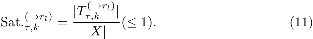
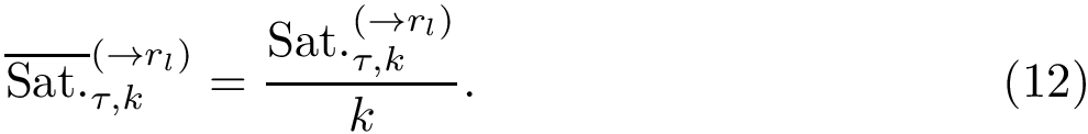
.) The saturation index at threshold is the fraction of sources present in  , that is:
In the absence of overlap between consecutive  , one would have
  . Thus, normalizing by provides a measure of the overlap between consecutive sets.
We note in passing that the previous sets can be used to define how many hits in a given reference list of genes  are obtained:
. The number of hits for particular values  is the size of the set
  . For a fixed , we similarly defined the size of the set
  .
.
Expression levels and fold-changes for genes in , MA plots. Two important quantities in transcriptomics are the expression level (mRNA count), and the expression changes, respectively denoted  and
and  on a logarithmic scale. The associated scatter plot is often called a MA plot.
Score radar plots. The difficulty in working with values  for
for  is that all pairs
  get mapped onto the same point. To get around this difficulty, we associate a radar plot with each point , yielding an overall score radar scatter plot.
Each gene score radar plot is defined as follows:
or ) log score observed for that gene. This background color makes it easy to spot the individual radar plots with high scores. (user defined) scores. and
and 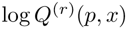 .
. Score radar scatter plot. Displaying all individual score radar plots in the plane yields the so-called Score radar scatter plot.
NB: While the Markov chain and score calculations in identifier-type agnostic, the generation of gene radars, and gene radar scatters, assumes that the identifiers used are protein identifiers, and could fail if another type of identifier is used.
Genes versus proteins. In the sequel, we manipulate genes and proteins. The following formats are used:
Protein Protein Interaction Network – PPIN. The PPIN file should be a tab-separated file of interactions, where each interaction has the two protein identifiers, and a weight ![$(0, 1]$](form_599.png) . This weights is morally the interaction probability – so that 0 amount to removing the edge.
. This weights is morally the interaction probability – so that 0 amount to removing the edge.
NB: These interactions are bidirectional ie give rise to arcs in both directions, whence two non null entries in the Markov chain transition matrix.
Gene set and target set . The Sources and Targets files are lists of protein identifiers, one per line.
Example: 5 sources used [65]
Example: 51 sources used [65]
Markov models and hit scores..
We compute hit scores (Def. def-hit-score) using the C++  library ([101] and Marmote).
For a given restart rate, we output a csv file containing the scores and  for all pairs in
  .
.
Example: results file for the whole MINT PPIN, obtained for  – see [65]
Reranked gene lists. Our final product is the set of top genes defined by (Def. def-genetrank), possibly accumulated over several values of the restart rate (Def. eq-topkler).
These set depend on three parameters:
used to compute the average score of a gene in of genes top-rankedWe output such lists in plain txt files.
Radar plots.
We assume a MA plot file, containing triples (gene id, logFC, logCPM).
The radar plots are obtained using this file and the reranked gene list file.
 |
| Example radar plot. |
 |
| The radar scatter plot combining the individual radar plots. |
The package proves two executables compiled from C++ programs, and three python scripts. We now briefly describe these programs, and refer the user to the Jupyter notebook for example calls.
C++ based executables.
 : program computing the transition matrices for the Markov chains representing the random walks (see [65] ).
 : program computing the hit probability vectors (Def. def-hit-proba-vector) computed from the transition matrices.
Python scripts.
 : script converting a list of gene ids into a list of protein ids, or vice versa.
 : script running the C++ based executables, and subsequently producing the file of hit scores, as well as the radar plots.
 : script exploiting the csv files containing all hit scores to compute the and the reranked gene lists.
As noticed above, Markov models rely on the C++ library [101], see Marmote
To use this package, proceed as follows:
and See the following jupyter notebook:
import os
import subprocess
import shutil
from SBL import SBL_pytools
from SBL_pytools import SBL_pytools as sblpyt

from SBL import SBL_Genetrank_application
from SBL_Genetrank_application import Genetrank_application

from SBL import SBL_Genetrank_gene_to_protein
from SBL_Genetrank_gene_to_protein import *
genes  = [line.rstrip() for line in open("data/proteins-targets-apoptosis-49-entries.in").readlines()]
print(genes)
translator = Genetrank_GeneProteinTranslator('hsapiens', direction='protein2gene')
translations = translator.translate(genes)
print(translations)
translations.summary()
['O43464', 'P19438', 'Q07817', 'O43521', 'D3DV04', 'P20333', 'Q13489', 'Q6FH21', 'P55211', 'O95831', 'Q13794', 'Q15628', 'Q8IX12', 'P98170', 'P55957', 'Q8WZ73', 'Q86W13', 'O14763', 'Q13618', 'Q07812', 'P62877', 'Q13546', 'Q9UMX3', 'P55210', 'O14798', 'Q9BXH1', 'O15392', 'Q13158', 'Q9NZS9', 'P21580', 'Q92843', 'O15519', 'P08574', 'P42575', 'P10415', 'O00198', 'O00220', 'Q92851', 'Q8WXG6', 'Q16611', 'Q13323', 'Q96LC9', 'Q13490', 'Q9NR28', 'P42574', 'Q14790', 'Q9UBN6', 'P25445', 'O14727']
Succesful Translations:
	O43464:	HTRA2
	P19438:	TNFRSF1A
	Q07817:	BCL2L1
	O43521:	BCL2L11
	P20333:	TNFRSF1B
	Q13489:	BIRC3
	P55211:	CASP9
	O95831:	AIFM1
	Q13794:	PMAIP1
	Q15628:	TRADD
	Q8IX12:	CCAR1
	P98170:	XIAP
	P55957:	BID
	Q8WZ73:	RFFL
	O14763:	TNFRSF10B
	Q13618:	CUL3
	Q07812:	BAX
	P62877:	RBX1
	Q13546:	RIPK1
	Q9UMX3:	BOK
	P55210:	CASP7
	O14798:	TNFRSF10C
	Q9BXH1:	BBC3
	O15392:	BIRC5
	Q13158:	FADD
	Q9NZS9:	BFAR
	P21580:	TNFAIP3
	Q92843:	BCL2L2
	O15519:	CFLAR
	P08574:	CYC1
	P42575:	CASP2
	P10415:	BCL2
	O00198:	HRK
	O00220:	TNFRSF10A
	Q92851:	CASP10
	Q8WXG6:	MADD
	Q16611:	BAK1
	Q13323:	BIK
	Q96LC9:	BMF
	Q13490:	BIRC2
	Q9NR28:	DIABLO
	P42574:	CASP3
	Q14790:	CASP8
	P25445:	FAS
	O14727:	APAF1
Ambiguous Translations:
Unable to Translate:
	D3DV04
	Q6FH21
	Q86W13
	Q9UBN6

Of 49 identifiers:
	45 successfully translated
	0 ambiguously translated
	4 unable to be translated
from SBL import SBL_Genetrank_application
from SBL_Genetrank_application import Genetrank_application
from SBL import SBL_pytools
from SBL_pytools import *

odir = "test5s"
if os.path.exists(odir):
    pass
    #os.system( ("rm -rf %s" % odir))
os.system( ("mkdir -p %s" % odir))

ppin_file_path = 'data/MINT-human-august2020.in'
sources_file_path = 'data/proteins-sources-5-entries.in'
targets_file_path = 'data/proteins-targets-apoptosis-49-entries.in'
pathways_dir_path = '/tmp/pathways'
os.mkdir(pathways_dir_path)

app = Genetrank_application(odir)
app.add_ppin_file(ppin_file_path)
app.add_sources_file(sources_file_path)
app.add_targets_file(targets_file_path)
app.add_pathways_dir(pathways_dir_path)
app.add_restart_probability(0.01)
app.add_restart_probability(0.3)

app.generate_inputs()
app.instantiate_simulations()
def odir_tree(highlight_pattern='^'):
    cmd = "tree %s | grep --color=always -e '^' -e '%s'" % (odir, highlight_pattern)
    tree = ''.join(os.popen(cmd).readlines())
    return tree
Uses the executable sbl-genetrank-Markov-models.exe to generate the Markov Chain .mcl transition matrix files to be used by MARMOTE. These files are one per source, named mcr_<internal_source_id>.mcl. markov_chain.mcl contains the normalization Markov Chain's transition matrix.
source_idx.txt, target_idx.txt, and map_protein_name_idx.txt are also produced to be used to cross-reference the identifiers used internally by the executable with the protein identifiers.
app.generate_markov_chains()

print(odir_tree('*.mcl'))
Creating directory for r=0.01 (cmd=mkdir -p test5s/r0.01)
Creating directory for r=0.30 (cmd=mkdir -p test5s/r0.30)

Generating Markov Chains (one for each source)...

	PPIN = MINT-human-august2020
	SOURCES = proteins-sources-5-entries
	TARGETS = proteins-targets-apoptosis-49-entries
	r = 0.01
	Running cmd=/home/asq/Dev/inria/projects/sbl/Applications/Genetrank/src/build/sbl-genetrank-Markov-models.exe -g data/MINT-human-august2020.in -p /tmp/pathways -s data/proteins-sources-5-entries.in -t data/proteins-targets-apoptosis-49-entries.in -r 0.01 -o test5s/r0.01


Generating Markov Chains (one for each source)...
	PPIN = MINT-human-august2020
	SOURCES = proteins-sources-5-entries
	TARGETS = proteins-targets-apoptosis-49-entries
	r = 0.30
	Running cmd=/home/asq/Dev/inria/projects/sbl/Applications/Genetrank/src/build/sbl-genetrank-Markov-models.exe -g data/MINT-human-august2020.in -p /tmp/pathways -s data/proteins-sources-5-entries.in -t data/proteins-targets-apoptosis-49-entries.in -r 0.30 -o test5s/r0.30
...Markov Chains generated.
(they can be found at test5s/r0.30/MINT-human-august2020_proteins-sources-5-entries_proteins-targets-apoptosis-49-entries_r0.30)


...Markov Chains generated.
(they can be found at test5s/r0.01/MINT-human-august2020_proteins-sources-5-entries_proteins-targets-apoptosis-49-entries_r0.01)


Creating directory for r=0.01 (cmd=mkdir -p test5s/r0.01)
Creating directory for r=0.30 (cmd=mkdir -p test5s/r0.30)


Generating Markov Chains (one for each source)...


Generating Markov Chains (one for each source)...	PPIN = MINT-human-august2020
	SOURCES = proteins-targets-apoptosis-49-entries
	TARGETS = proteins-sources-5-entries
	r = 0.01

	PPIN = MINT-human-august2020
	SOURCES = proteins-targets-apoptosis-49-entries
	TARGETS = proteins-sources-5-entries
	r = 0.30
	Running cmd=/home/asq/Dev/inria/projects/sbl/Applications/Genetrank/src/build/sbl-genetrank-Markov-models.exe -g data/MINT-human-august2020.in -p /tmp/pathways -s data/proteins-targets-apoptosis-49-entries.in -t data/proteins-sources-5-entries.in -r 0.01 -o test5s/r0.01	Running cmd=/home/asq/Dev/inria/projects/sbl/Applications/Genetrank/src/build/sbl-genetrank-Markov-models.exe -g data/MINT-human-august2020.in -p /tmp/pathways -s data/proteins-targets-apoptosis-49-entries.in -t data/proteins-sources-5-entries.in -r 0.30 -o test5s/r0.30

...Markov Chains generated.
(they can be found at test5s/r0.30/MINT-human-august2020_proteins-targets-apoptosis-49-entries_proteins-sources-5-entries_r0.30)


...Markov Chains generated.
(they can be found at test5s/r0.01/MINT-human-august2020_proteins-targets-apoptosis-49-entries_proteins-sources-5-entries_r0.01)


test5s
├── figures
│   └── r0.30
├── r0.01
│   ├── MINT-human-august2020_proteins-sources-5-entries_proteins-targets-apoptosis-49-entries_r0.01
│   │   ├── map_protein_name_idx.txt
│   │   ├── markov_chain.mcl
│   │   ├── mcr_2437.mcl
│   │   ├── mcr_3187.mcl
│   │   ├── mcr_3480.mcl
│   │   ├── mcr_420.mcl
│   │   ├── mcr_679.mcl
│   │   ├── source_idx.txt
│   │   ├── source_names.txt
│   │   └── target_idx.txt
│   └── MINT-human-august2020_proteins-targets-apoptosis-49-entries_proteins-sources-5-entries_r0.01
│       ├── map_protein_name_idx.txt
│       ├── markov_chain.mcl
│       ├── mcr_10406.mcl
│       ├── mcr_10715.mcl
│       ├── mcr_1560.mcl
│       ├── mcr_2123.mcl
│       ├── mcr_2292.mcl
│       ├── mcr_2743.mcl
│       ├── mcr_2777.mcl
│       ├── mcr_2823.mcl
│       ├── mcr_2995.mcl
│       ├── mcr_3584.mcl
│       ├── mcr_3585.mcl
│       ├── mcr_385.mcl
│       ├── mcr_4131.mcl
│       ├── mcr_4132.mcl
│       ├── mcr_4158.mcl
│       ├── mcr_4407.mcl
│       ├── mcr_4686.mcl
│       ├── mcr_4930.mcl
│       ├── mcr_4932.mcl
│       ├── mcr_5157.mcl
│       ├── mcr_5201.mcl
│       ├── mcr_5251.mcl
│       ├── mcr_5252.mcl
│       ├── mcr_5266.mcl
│       ├── mcr_5296.mcl
│       ├── mcr_5326.mcl
│       ├── mcr_5499.mcl
│       ├── mcr_551.mcl
│       ├── mcr_560.mcl
│       ├── mcr_5668.mcl
│       ├── mcr_5770.mcl
│       ├── mcr_699.mcl
│       ├── mcr_722.mcl
│       ├── mcr_7333.mcl
│       ├── mcr_8055.mcl
│       ├── mcr_8223.mcl
│       ├── mcr_8226.mcl
│       ├── mcr_858.mcl
│       ├── mcr_868.mcl
│       ├── mcr_9210.mcl
│       ├── mcr_9945.mcl
│       ├── source_idx.txt
│       ├── source_names.txt
│       └── target_idx.txt
└── r0.30
    ├── MINT-human-august2020_proteins-sources-5-entries_proteins-targets-apoptosis-49-entries_r0.30
    │   ├── map_protein_name_idx.txt
    │   ├── markov_chain.mcl
    │   ├── mcr_2437.mcl
    │   ├── mcr_3187.mcl
    │   ├── mcr_3480.mcl
    │   ├── mcr_420.mcl
    │   ├── mcr_679.mcl
    │   ├── source_idx.txt
    │   ├── source_names.txt
    │   └── target_idx.txt
    └── MINT-human-august2020_proteins-targets-apoptosis-49-entries_proteins-sources-5-entries_r0.30
        ├── map_protein_name_idx.txt
        ├── markov_chain.mcl
        ├── mcr_10406.mcl
        ├── mcr_10715.mcl
        ├── mcr_1560.mcl
        ├── mcr_2123.mcl
        ├── mcr_2292.mcl
        ├── mcr_2743.mcl
        ├── mcr_2777.mcl
        ├── mcr_2823.mcl
        ├── mcr_2995.mcl
        ├── mcr_3584.mcl
        ├── mcr_3585.mcl
        ├── mcr_385.mcl
        ├── mcr_4131.mcl
        ├── mcr_4132.mcl
        ├── mcr_4158.mcl
        ├── mcr_4407.mcl
        ├── mcr_4686.mcl
        ├── mcr_4930.mcl
        ├── mcr_4932.mcl
        ├── mcr_5157.mcl
        ├── mcr_5201.mcl
        ├── mcr_5251.mcl
        ├── mcr_5252.mcl
        ├── mcr_5266.mcl
        ├── mcr_5296.mcl
        ├── mcr_5326.mcl
        ├── mcr_5499.mcl
        ├── mcr_551.mcl
        ├── mcr_560.mcl
        ├── mcr_5668.mcl
        ├── mcr_5770.mcl
        ├── mcr_699.mcl
        ├── mcr_722.mcl
        ├── mcr_7333.mcl
        ├── mcr_8055.mcl
        ├── mcr_8223.mcl
        ├── mcr_8226.mcl
        ├── mcr_858.mcl
        ├── mcr_868.mcl
        ├── mcr_9210.mcl
        ├── mcr_9945.mcl
        ├── source_idx.txt
        ├── source_names.txt
        └── target_idx.txt

8 directories, 112 files
Uses the executable sbl-genetrank-hit-probabilities.exe to calculate the pairwise hit probabilities which are written to hit-vectors.txt and the centrality for normalization, written to normalization-distribution.txt
app.calculate_hit_probabilities()

print(odir_tree())
Calculating Hit Probability Vectors...


Calculating Hit Probability Vectors...
	PPIN = MINT-human-august2020
	SOURCES = proteins-sources-5-entries
	TARGETS = proteins-targets-apoptosis-49-entries
	r = 0.30	PPIN = MINT-human-august2020
	SOURCES = proteins-sources-5-entries
	TARGETS = proteins-targets-apoptosis-49-entries
	r = 0.01
	Running cmd=/home/asq/Dev/inria/projects/sbl/Applications/Genetrank/src/build/sbl-genetrank-hit-probabilities.exe -i test5s/r0.30/MINT-human-august2020_proteins-sources-5-entries_proteins-targets-apoptosis-49-entries_r0.30 -o test5s/r0.30/MINT-human-august2020_proteins-sources-5-entries_proteins-targets-apoptosis-49-entries_r0.30 | grep Status

	Running cmd=/home/asq/Dev/inria/projects/sbl/Applications/Genetrank/src/build/sbl-genetrank-hit-probabilities.exe -i test5s/r0.01/MINT-human-august2020_proteins-sources-5-entries_proteins-targets-apoptosis-49-entries_r0.01 -o test5s/r0.01/MINT-human-august2020_proteins-sources-5-entries_proteins-targets-apoptosis-49-entries_r0.01 | grep Status
...Hit Probabilities Calculated.
   Source  Target  Hit Probability
0  O00429  O00220         0.002966
1  O15304  O00220         0.003361
2  P13196  O00220         0.003144
3  P30050  O00220         0.003933
4  P38919  O00220         0.003893


...Hit Probabilities Calculated.
   Source  Target  Hit Probability
0  O00429  O00220         0.001218
1  O15304  O00220         0.003362
2  P13196  O00220         0.001755
3  P30050  O00220         0.011149
4  P38919  O00220         0.015557


Calculating Hit Probability Vectors...
	PPIN = MINT-human-august2020
	SOURCES = proteins-targets-apoptosis-49-entries
	TARGETS = proteins-sources-5-entries
	r = 0.01
	Running cmd=/home/asq/Dev/inria/projects/sbl/Applications/Genetrank/src/build/sbl-genetrank-hit-probabilities.exe -i test5s/r0.01/MINT-human-august2020_proteins-targets-apoptosis-49-entries_proteins-sources-5-entries_r0.01 -o test5s/r0.01/MINT-human-august2020_proteins-targets-apoptosis-49-entries_proteins-sources-5-entries_r0.01 | grep Status

Calculating Hit Probability Vectors...

	PPIN = MINT-human-august2020
	SOURCES = proteins-targets-apoptosis-49-entries
	TARGETS = proteins-sources-5-entries
	r = 0.30
	Running cmd=/home/asq/Dev/inria/projects/sbl/Applications/Genetrank/src/build/sbl-genetrank-hit-probabilities.exe -i test5s/r0.30/MINT-human-august2020_proteins-targets-apoptosis-49-entries_proteins-sources-5-entries_r0.30 -o test5s/r0.30/MINT-human-august2020_proteins-targets-apoptosis-49-entries_proteins-sources-5-entries_r0.30 | grep Status
...Hit Probabilities Calculated.
   Source  Target  Hit Probability
0  O00429  O00220         0.130106
1  O15304  O00220         0.020702
2  P13196  O00220         0.234095
3  P30050  O00220         0.293829
4  P38919  O00220         0.320440


...Hit Probabilities Calculated.
   Source  Target  Hit Probability
0  O00429  O00220         0.078315
1  O15304  O00220         0.005530
2  P13196  O00220         0.076769
3  P30050  O00220         0.419885
4  P38919  O00220         0.417971


test5s
├── figures
│   └── r0.30
├── r0.01
│   ├── MINT-human-august2020_proteins-sources-5-entries_proteins-targets-apoptosis-49-entries_r0.01
│   │   ├── hit-vectors.txt
│   │   ├── map_protein_name_idx.txt
│   │   ├── markov_chain.mcl
│   │   ├── mcr_2437.mcl
│   │   ├── mcr_3187.mcl
│   │   ├── mcr_3480.mcl
│   │   ├── mcr_420.mcl
│   │   ├── mcr_679.mcl
│   │   ├── normalization-distribution.txt
│   │   ├── source_idx.txt
│   │   ├── source_names.txt
│   │   └── target_idx.txt
│   └── MINT-human-august2020_proteins-targets-apoptosis-49-entries_proteins-sources-5-entries_r0.01
│       ├── hit-vectors.txt
│       ├── map_protein_name_idx.txt
│       ├── markov_chain.mcl
│       ├── mcr_10406.mcl
│       ├── mcr_10715.mcl
│       ├── mcr_1560.mcl
│       ├── mcr_2123.mcl
│       ├── mcr_2292.mcl
│       ├── mcr_2743.mcl
│       ├── mcr_2777.mcl
│       ├── mcr_2823.mcl
│       ├── mcr_2995.mcl
│       ├── mcr_3584.mcl
│       ├── mcr_3585.mcl
│       ├── mcr_385.mcl
│       ├── mcr_4131.mcl
│       ├── mcr_4132.mcl
│       ├── mcr_4158.mcl
│       ├── mcr_4407.mcl
│       ├── mcr_4686.mcl
│       ├── mcr_4930.mcl
│       ├── mcr_4932.mcl
│       ├── mcr_5157.mcl
│       ├── mcr_5201.mcl
│       ├── mcr_5251.mcl
│       ├── mcr_5252.mcl
│       ├── mcr_5266.mcl
│       ├── mcr_5296.mcl
│       ├── mcr_5326.mcl
│       ├── mcr_5499.mcl
│       ├── mcr_551.mcl
│       ├── mcr_560.mcl
│       ├── mcr_5668.mcl
│       ├── mcr_5770.mcl
│       ├── mcr_699.mcl
│       ├── mcr_722.mcl
│       ├── mcr_7333.mcl
│       ├── mcr_8055.mcl
│       ├── mcr_8223.mcl
│       ├── mcr_8226.mcl
│       ├── mcr_858.mcl
│       ├── mcr_868.mcl
│       ├── mcr_9210.mcl
│       ├── mcr_9945.mcl
│       ├── normalization-distribution.txt
│       ├── source_idx.txt
│       ├── source_names.txt
│       └── target_idx.txt
└── r0.30
    ├── MINT-human-august2020_proteins-sources-5-entries_proteins-targets-apoptosis-49-entries_r0.30
    │   ├── hit-vectors.txt
    │   ├── map_protein_name_idx.txt
    │   ├── markov_chain.mcl
    │   ├── mcr_2437.mcl
    │   ├── mcr_3187.mcl
    │   ├── mcr_3480.mcl
    │   ├── mcr_420.mcl
    │   ├── mcr_679.mcl
    │   ├── normalization-distribution.txt
    │   ├── source_idx.txt
    │   ├── source_names.txt
    │   └── target_idx.txt
    └── MINT-human-august2020_proteins-targets-apoptosis-49-entries_proteins-sources-5-entries_r0.30
        ├── hit-vectors.txt
        ├── map_protein_name_idx.txt
        ├── markov_chain.mcl
        ├── mcr_10406.mcl
        ├── mcr_10715.mcl
        ├── mcr_1560.mcl
        ├── mcr_2123.mcl
        ├── mcr_2292.mcl
        ├── mcr_2743.mcl
        ├── mcr_2777.mcl
        ├── mcr_2823.mcl
        ├── mcr_2995.mcl
        ├── mcr_3584.mcl
        ├── mcr_3585.mcl
        ├── mcr_385.mcl
        ├── mcr_4131.mcl
        ├── mcr_4132.mcl
        ├── mcr_4158.mcl
        ├── mcr_4407.mcl
        ├── mcr_4686.mcl
        ├── mcr_4930.mcl
        ├── mcr_4932.mcl
        ├── mcr_5157.mcl
        ├── mcr_5201.mcl
        ├── mcr_5251.mcl
        ├── mcr_5252.mcl
        ├── mcr_5266.mcl
        ├── mcr_5296.mcl
        ├── mcr_5326.mcl
        ├── mcr_5499.mcl
        ├── mcr_551.mcl
        ├── mcr_560.mcl
        ├── mcr_5668.mcl
        ├── mcr_5770.mcl
        ├── mcr_699.mcl
        ├── mcr_722.mcl
        ├── mcr_7333.mcl
        ├── mcr_8055.mcl
        ├── mcr_8223.mcl
        ├── mcr_8226.mcl
        ├── mcr_858.mcl
        ├── mcr_868.mcl
        ├── mcr_9210.mcl
        ├── mcr_9945.mcl
        ├── normalization-distribution.txt
        ├── source_idx.txt
        ├── source_names.txt
        └── target_idx.txt

8 directories, 120 files
Scores are calculated by the Genetrank_simulation_result class within SBL_Genetrank_simulation.py using the results from the previous step. Pairwise scores are written to <sources_file_name>_<targets_file_name>_pairwise_scores.csv
app.calculate_scores()

print(odir_tree())
test5s
├── figures
│   └── r0.30
├── r0.01
│   ├── MINT-human-august2020_proteins-sources-5-entries_proteins-targets-apoptosis-49-entries_r0.01
│   │   ├── hit-vectors.txt
│   │   ├── map_protein_name_idx.txt
│   │   ├── markov_chain.mcl
│   │   ├── mcr_2437.mcl
│   │   ├── mcr_3187.mcl
│   │   ├── mcr_3480.mcl
│   │   ├── mcr_420.mcl
│   │   ├── mcr_679.mcl
│   │   ├── normalization-distribution.txt
│   │   ├── source_idx.txt
│   │   ├── source_names.txt
│   │   └── target_idx.txt
│   ├── MINT-human-august2020_proteins-targets-apoptosis-49-entries_proteins-sources-5-entries_r0.01
│   │   ├── hit-vectors.txt
│   │   ├── map_protein_name_idx.txt
│   │   ├── markov_chain.mcl
│   │   ├── mcr_10406.mcl
│   │   ├── mcr_10715.mcl
│   │   ├── mcr_1560.mcl
│   │   ├── mcr_2123.mcl
│   │   ├── mcr_2292.mcl
│   │   ├── mcr_2743.mcl
│   │   ├── mcr_2777.mcl
│   │   ├── mcr_2823.mcl
│   │   ├── mcr_2995.mcl
│   │   ├── mcr_3584.mcl
│   │   ├── mcr_3585.mcl
│   │   ├── mcr_385.mcl
│   │   ├── mcr_4131.mcl
│   │   ├── mcr_4132.mcl
│   │   ├── mcr_4158.mcl
│   │   ├── mcr_4407.mcl
│   │   ├── mcr_4686.mcl
│   │   ├── mcr_4930.mcl
│   │   ├── mcr_4932.mcl
│   │   ├── mcr_5157.mcl
│   │   ├── mcr_5201.mcl
│   │   ├── mcr_5251.mcl
│   │   ├── mcr_5252.mcl
│   │   ├── mcr_5266.mcl
│   │   ├── mcr_5296.mcl
│   │   ├── mcr_5326.mcl
│   │   ├── mcr_5499.mcl
│   │   ├── mcr_551.mcl
│   │   ├── mcr_560.mcl
│   │   ├── mcr_5668.mcl
│   │   ├── mcr_5770.mcl
│   │   ├── mcr_699.mcl
│   │   ├── mcr_722.mcl
│   │   ├── mcr_7333.mcl
│   │   ├── mcr_8055.mcl
│   │   ├── mcr_8223.mcl
│   │   ├── mcr_8226.mcl
│   │   ├── mcr_858.mcl
│   │   ├── mcr_868.mcl
│   │   ├── mcr_9210.mcl
│   │   ├── mcr_9945.mcl
│   │   ├── normalization-distribution.txt
│   │   ├── source_idx.txt
│   │   ├── source_names.txt
│   │   └── target_idx.txt
│   └── proteins-sources-5-entries_proteins-targets-apoptosis-49-entries-pairwise_scores.csv
└── r0.30
    ├── MINT-human-august2020_proteins-sources-5-entries_proteins-targets-apoptosis-49-entries_r0.30
    │   ├── hit-vectors.txt
    │   ├── map_protein_name_idx.txt
    │   ├── markov_chain.mcl
    │   ├── mcr_2437.mcl
    │   ├── mcr_3187.mcl
    │   ├── mcr_3480.mcl
    │   ├── mcr_420.mcl
    │   ├── mcr_679.mcl
    │   ├── normalization-distribution.txt
    │   ├── source_idx.txt
    │   ├── source_names.txt
    │   └── target_idx.txt
    ├── MINT-human-august2020_proteins-targets-apoptosis-49-entries_proteins-sources-5-entries_r0.30
    │   ├── hit-vectors.txt
    │   ├── map_protein_name_idx.txt
    │   ├── markov_chain.mcl
    │   ├── mcr_10406.mcl
    │   ├── mcr_10715.mcl
    │   ├── mcr_1560.mcl
    │   ├── mcr_2123.mcl
    │   ├── mcr_2292.mcl
    │   ├── mcr_2743.mcl
    │   ├── mcr_2777.mcl
    │   ├── mcr_2823.mcl
    │   ├── mcr_2995.mcl
    │   ├── mcr_3584.mcl
    │   ├── mcr_3585.mcl
    │   ├── mcr_385.mcl
    │   ├── mcr_4131.mcl
    │   ├── mcr_4132.mcl
    │   ├── mcr_4158.mcl
    │   ├── mcr_4407.mcl
    │   ├── mcr_4686.mcl
    │   ├── mcr_4930.mcl
    │   ├── mcr_4932.mcl
    │   ├── mcr_5157.mcl
    │   ├── mcr_5201.mcl
    │   ├── mcr_5251.mcl
    │   ├── mcr_5252.mcl
    │   ├── mcr_5266.mcl
    │   ├── mcr_5296.mcl
    │   ├── mcr_5326.mcl
    │   ├── mcr_5499.mcl
    │   ├── mcr_551.mcl
    │   ├── mcr_560.mcl
    │   ├── mcr_5668.mcl
    │   ├── mcr_5770.mcl
    │   ├── mcr_699.mcl
    │   ├── mcr_722.mcl
    │   ├── mcr_7333.mcl
    │   ├── mcr_8055.mcl
    │   ├── mcr_8223.mcl
    │   ├── mcr_8226.mcl
    │   ├── mcr_858.mcl
    │   ├── mcr_868.mcl
    │   ├── mcr_9210.mcl
    │   ├── mcr_9945.mcl
    │   ├── normalization-distribution.txt
    │   ├── source_idx.txt
    │   ├── source_names.txt
    │   └── target_idx.txt
    └── proteins-sources-5-entries_proteins-targets-apoptosis-49-entries-pairwise_scores.csv

8 directories, 122 files
from SBL import SBL_Genetrank_simulation_statistics
from SBL_Genetrank_simulation_statistics import Genetrank_simulation_visualizations

r03_simulation = app.get_simulation(ppin_file_path, sources_file_path, targets_file_path, pathways_dir_path, 0.3)
r03_simulation_visualizations = Genetrank_simulation_visualizations(r03_simulation)
r03_simulation_visualizations.generate_gene_score_radar('SIVA1', show=True)

app.logFC_logCPM_file = 'data/CellFate-LogCPM-LogFC-pval-FDR-mmc4.xls'
app.generate_gene_score_radar_scatter_plots()

print(odir_tree())
findfont: Font family ['normal'] not found. Falling back to DejaVu Sans.
findfont: Font family ['normal'] not found. Falling back to DejaVu Sans.
findfont: Font family ['normal'] not found. Falling back to DejaVu Sans.
findfont: Font family ['normal'] not found. Falling back to DejaVu Sans.
findfont: Font family ['normal'] not found. Falling back to DejaVu Sans.
test5s
├── figures
│   ├── r0.01
│   │   └── score_radar_scatter.pdf
│   └── r0.30
│       └── score_radar_scatter.pdf
├── r0.01
│   ├── MINT-human-august2020_proteins-sources-5-entries_proteins-targets-apoptosis-49-entries_r0.01
│   │   ├── hit-vectors.txt
│   │   ├── map_protein_name_idx.txt
│   │   ├── markov_chain.mcl
│   │   ├── mcr_2437.mcl
│   │   ├── mcr_3187.mcl
│   │   ├── mcr_3480.mcl
│   │   ├── mcr_420.mcl
│   │   ├── mcr_679.mcl
│   │   ├── normalization-distribution.txt
│   │   ├── source_idx.txt
│   │   ├── source_names.txt
│   │   └── target_idx.txt
│   ├── MINT-human-august2020_proteins-targets-apoptosis-49-entries_proteins-sources-5-entries_r0.01
│   │   ├── hit-vectors.txt
│   │   ├── map_protein_name_idx.txt
│   │   ├── markov_chain.mcl
│   │   ├── mcr_10406.mcl
│   │   ├── mcr_10715.mcl
│   │   ├── mcr_1560.mcl
│   │   ├── mcr_2123.mcl
│   │   ├── mcr_2292.mcl
│   │   ├── mcr_2743.mcl
│   │   ├── mcr_2777.mcl
│   │   ├── mcr_2823.mcl
│   │   ├── mcr_2995.mcl
│   │   ├── mcr_3584.mcl
│   │   ├── mcr_3585.mcl
│   │   ├── mcr_385.mcl
│   │   ├── mcr_4131.mcl
│   │   ├── mcr_4132.mcl
│   │   ├── mcr_4158.mcl
│   │   ├── mcr_4407.mcl
│   │   ├── mcr_4686.mcl
│   │   ├── mcr_4930.mcl
│   │   ├── mcr_4932.mcl
│   │   ├── mcr_5157.mcl
│   │   ├── mcr_5201.mcl
│   │   ├── mcr_5251.mcl
│   │   ├── mcr_5252.mcl
│   │   ├── mcr_5266.mcl
│   │   ├── mcr_5296.mcl
│   │   ├── mcr_5326.mcl
│   │   ├── mcr_5499.mcl
│   │   ├── mcr_551.mcl
│   │   ├── mcr_560.mcl
│   │   ├── mcr_5668.mcl
│   │   ├── mcr_5770.mcl
│   │   ├── mcr_699.mcl
│   │   ├── mcr_722.mcl
│   │   ├── mcr_7333.mcl
│   │   ├── mcr_8055.mcl
│   │   ├── mcr_8223.mcl
│   │   ├── mcr_8226.mcl
│   │   ├── mcr_858.mcl
│   │   ├── mcr_868.mcl
│   │   ├── mcr_9210.mcl
│   │   ├── mcr_9945.mcl
│   │   ├── normalization-distribution.txt
│   │   ├── source_idx.txt
│   │   ├── source_names.txt
│   │   └── target_idx.txt
│   └── proteins-sources-5-entries_proteins-targets-apoptosis-49-entries-pairwise_scores.csv
└── r0.30
    ├── MINT-human-august2020_proteins-sources-5-entries_proteins-targets-apoptosis-49-entries_r0.30
    │   ├── hit-vectors.txt
    │   ├── map_protein_name_idx.txt
    │   ├── markov_chain.mcl
    │   ├── mcr_2437.mcl
    │   ├── mcr_3187.mcl
    │   ├── mcr_3480.mcl
    │   ├── mcr_420.mcl
    │   ├── mcr_679.mcl
    │   ├── normalization-distribution.txt
    │   ├── source_idx.txt
    │   ├── source_names.txt
    │   └── target_idx.txt
    ├── MINT-human-august2020_proteins-targets-apoptosis-49-entries_proteins-sources-5-entries_r0.30
    │   ├── hit-vectors.txt
    │   ├── map_protein_name_idx.txt
    │   ├── markov_chain.mcl
    │   ├── mcr_10406.mcl
    │   ├── mcr_10715.mcl
    │   ├── mcr_1560.mcl
    │   ├── mcr_2123.mcl
    │   ├── mcr_2292.mcl
    │   ├── mcr_2743.mcl
    │   ├── mcr_2777.mcl
    │   ├── mcr_2823.mcl
    │   ├── mcr_2995.mcl
    │   ├── mcr_3584.mcl
    │   ├── mcr_3585.mcl
    │   ├── mcr_385.mcl
    │   ├── mcr_4131.mcl
    │   ├── mcr_4132.mcl
    │   ├── mcr_4158.mcl
    │   ├── mcr_4407.mcl
    │   ├── mcr_4686.mcl
    │   ├── mcr_4930.mcl
    │   ├── mcr_4932.mcl
    │   ├── mcr_5157.mcl
    │   ├── mcr_5201.mcl
    │   ├── mcr_5251.mcl
    │   ├── mcr_5252.mcl
    │   ├── mcr_5266.mcl
    │   ├── mcr_5296.mcl
    │   ├── mcr_5326.mcl
    │   ├── mcr_5499.mcl
    │   ├── mcr_551.mcl
    │   ├── mcr_560.mcl
    │   ├── mcr_5668.mcl
    │   ├── mcr_5770.mcl
    │   ├── mcr_699.mcl
    │   ├── mcr_722.mcl
    │   ├── mcr_7333.mcl
    │   ├── mcr_8055.mcl
    │   ├── mcr_8223.mcl
    │   ├── mcr_8226.mcl
    │   ├── mcr_858.mcl
    │   ├── mcr_868.mcl
    │   ├── mcr_9210.mcl
    │   ├── mcr_9945.mcl
    │   ├── normalization-distribution.txt
    │   ├── source_idx.txt
    │   ├── source_names.txt
    │   └── target_idx.txt
    └── proteins-sources-5-entries_proteins-targets-apoptosis-49-entries-pairwise_scores.csv

9 directories, 124 files
Unless stated otherwise, packages of the SBL are distributed under the following specific license SBL license.
The package, however, is distributed under the Apache 2.0 License.