|
Structural Bioinformatics Library
Template C++ / Python API for developping structural bioinformatics applications.
|
|
Structural Bioinformatics Library
Template C++ / Python API for developping structural bioinformatics applications.
|
Authors: D. Agarwal and C. Caillouet and F. Cazals and D. Coudert
![]()
Connectivity inference (CI). Consider a macro-molecular assembly consisting of subunits (typically proteins or nucleic acids). Assume that these subunits are known, but that the pairwise contacts between them are not. Connectivity Inference (CI) aims at inferring these unknown contacts (Fig fig-lego-example).
To address CI, let an oligomer be a small assembly dissociated from the intact assembly. An oligomer formula is the list of subunits involved in an oligomer. That is, an oligomer formula is the description of the composition of the oligomer, giving the number of instances of each molecule. We define a connectivity inference specification (specification for short) as a list of oligomers.
Oligomers typically come from native mass spectrometry experiments on a solution containing the assembly of interest, under various experimental conditions [180]. In particular, stringent conditions (e.g. low pH) result in complete dissociation of the assembly, so that the individual molecules are identified, while less stringent conditions result in the disruption of the assembly into multiple overlapping complexes.
Additionally, one may use an interaction likelihood qualifying the plausibility of the interaction of two subunits. On the experimental side, various assays have been developed to check whether two proteins interact, including yeast-two-hybrid, mammalian protein-protein interaction trap, luminescence-based mammalian interactome, yellow fluorescent protein complementation assay, etc. [31]. On the in silico side, various interactions attributes can be used, such as gene expressions patterns (proteins with identical patterns are more likely to interact), domain interaction data (a known interaction between two domains hints at an interaction between proteins containing these domains), common neighbors in protein-protein interaction networks, or bibliographical data (number of publications providing evidence for a particular interaction).
We view a CI problem as a problem on an unknown graph 
This application provides algorithms solving CI problems, in the following sense:

We actually provide two ways to solve CI problems:
Unweighted case and MCI problems. In this setting, the input consists of the list of subunits, of a list of oligomers, and possibly labels to enforce/forbid contacts. The output consists of a list of solutions. Again, note that in general, the solution is not unique.
We wish to find solutions without speculating on the unknown number of contacts in the assembly. We therefore define the Minimum Connectivity Inference problem (MCI) as a variant of CI such that valid edge sets of minimum cardinality are sought. This cardinality is denoted 
Weighted case and MWCI problems. Assume, as discussed above, that one also has an interaction likelihood, namely a number in the range ![$[0,1]$](form_322_dark.png)
![$\alpha\in [0,1]$](form_323_dark.png)

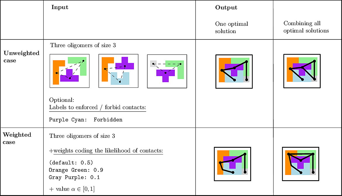 |
MCI and MWCI Toy Examples Note that in addition to the oligomers, the input may also involve labels to enforce/forbid contacts. Bottom row: the weighted case In addition to oligomers, one may specify weights to favor/unfavor specific contacts. A value |
We illustrate the input and output of a CI problem on our simple lego problem (Fig. fig-lego-example). The reader is referred to the subsequent section for further details.
The CI problem is specified by the list of subunits and oligomers:

Upon running the following command:
> sbl-mwci.py -f ../demos/data/lego-example.txt -c
One gets the list of two optimal solutions:

In this section, we formally define the MCI problem, and show how to process a real example, the yeast exosome (Fig. fig-yeast-exosome).
Consider a set of oligomers 

To specify the first option (which is the default one), consider a given oligomer 


The second option consists of annotating the edges from the default option: selected edges are forbidden, selected edges are enforced, the remaining ones are possible. This specification is achieved by means of one label per edge:
F: forbidden.
E: enforced (NB: this is equivalent to specifying a dimer containing these two subunits).
While enforcing edges is natural when two subunits are known to interact, the possibility to rule out edges is also frequently used. One common situation is the connectivity inference for an assembly for which a cryo-EM map is known, and for which two subunits can be located in the map without ambiguity. If these subunits are located far apart, then, the corresponding edge should be forbidden.
The specification of labels also makes it possible to specify the possible neighbors of a given subunit by ruling out selected edges involving that subunit.
As noticed above, a MCI problem does not admit, in general, a unique solution. Therefore, our strategy consists of enumerating all optimal solutions, from which various pieces of information are returned to the user. We define:

Sensitivity, specificity, coverage. Connectivity inference problems are generally solved when contacts are sought. On the other hand, reference contacts may have been obtained from biophysical and biochemical experiments such as x-ray crystallography, tandem mass spectrometry or cross linking experiments. We denote 
The reference set 


Positives ( 


Note that specificity requires the set 
We also combine the previous values to define the following coverage score, which favors true positives, penalizes false positives and false negatives, and scales the results with respect to the total number of reference contacts (since

Note that the maximum value is one, and that the coverage score may be negative.
Signed Contact score. Given a set of reference contacts, the signed contact score is the contact score multiplied by 

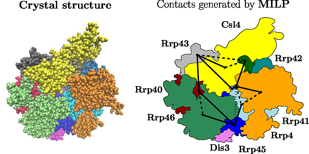 |
The Yeast Exosome (Left) Crystal structure (Right) The solid edges reported by the program |
The options offered by the program 
To solve MCI and analyze the resulting solutions, one runs:
> sbl-mwci.py -f demos/data/yeast-exosome-without-Csl4-mwci-spec.txt -c -a
The specification of the yeast exosome, with selected labeled contacts, is accessible from the specification file in Table table-mwci-without-ref-input-files .
| File Name | Description |
| MWCI Specification File | Does not contain the reference contacts |
If in addition one wishes to compare the solutions returned against a set of reference contacts, in order to compute signed contact scores instead of scores, the specification file must contains these reference contacts – see Table table-mwci-with-ref-input-files :
> sbl-mwci.py -f demos/data/yeast-exosome-without-Csl4-mwci-spec-with-ref.txt -c -a
Note that computation of solutions were already done, so that they are skipped by automatically loading them from an output serialized archive (json file format).
| File Name | Description |
| MWCI Specification File | Contains the reference contacts |
For the first command line above, one gets files containing:
| Preview | File Name | Description |
| Solutions File (txt) | File summaring the solutions | |
| Solutions File (json) | Serialized archive of solutions | |
| Consensus Solutions File | File summaring the consensus solutions | |
| Contact Scores Plot | Distribution of contacts' scores, see Fig. fig-contact-scores-yeast-exosome-without-Csl4 | |
| Consensus Contact Scores Plot | Distribution of consensus contacts' scores, see Fig. fig-contact-scores-yeast-exosome-without-Csl4 |
With respect to the previous call, the following new files are generated:
| Preview | File Name | Description |
| Contacts Assessments | Assessment of contacts (sensitivity, specificity and coverage score) | |
| Consensus Contacts Assessments | Assessment of consensus contacts (sensitivity, specificity and coverage score) | |
| Contact Signed Scores Plot | Distribution of contacts' signed scores, see Fig. fig-signed-contact-scores-yeast-exosome-without-Csl4 | |
| Consensus Contact Signed Scores Plot | Distribution of consensus contacts' signed scores, see Fig. fig-signed-contact-scores-yeast-exosome-without-Csl4 |
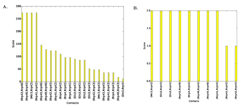 |
| Contact scores for Yeast Exosome (w/o Csl4) A. Contact scores in the set of solutions B. Scores for consensus contacts |
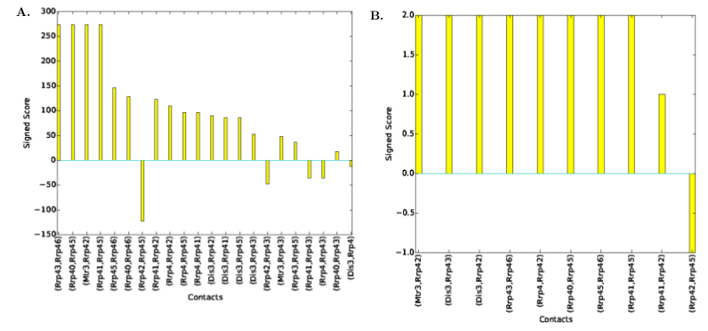 |
| Signed scores of contacts for Yeast Exosome (without Csl4) with reference set of contacts A. Signed contact scores in the set of solutions B. Signed scores for consensus contacts |

Assume that each candidate edge 
![$w(e)\in
[0,1]$](form_348_dark.png)
![$\alpha \in
[0,1]$](form_349_dark.png)

Thus, in solving an MWCI problem, we wish to find solutions minimizing the sum of such weights for all edges of the solution. All edges from the pool may carry a weight. Depending on which weights are specified, we proceed as follows:
Edges with a weight specified: that weight is used
The following remarks are in order regarding labels versus weights:


Below, we show how to process the yeast exosome, with weights placed on selected edges – see Table table-mwci-weighted-input-files .
> sbl-mwci.py -f demos/data/yeast-exosome-without-Csl4-mwci-spec-with-ref-with-weights.txt -a -c --alpha 0.25
| File Name | Description |
| MWCI Specification File | With weights on selected contacts and reference contacts |
The output files of the run described in section Input: Specifications and File Types are listed in Table table-mwci-weighted-with-ref-output-files .
| Preview | File Name | Description |
| Solutions File (txt) | File summaring the solutions | |
| Solutions File (json) | Serialized archive of solutions | |
| Consensus Solutions File | File summaring the consensus solutions | |
| Contacts Assessments | Assessment of contacts (sensitivity, specificity and coverage score) | |
| Consensus Contacts Assessments | Assessment of consensus contacts (sensitivity, specificity and coverage score) | |
| Contact Scores Plot | Distribution of signed contacts' scores | |
| Consensus Contact Scores Plot | Distribution of signed consensus contacts' scores |
The set of consensus contacts computed on solving the MWCI is a backbone of the protein assembly. It has ben observed [2] that the consensus contacts are small in number but are characterized by high specificity which is of great interest from strucutral point of view. We therefore seek to extend the set of initial set of consensus contacts using a bootstrapping procedure which iteratively forbids one consensus contact, so a to trigger a rewiring of the solutions:
The command line to activate the bootstrapping procedure includes "-b" option as shown below:
> sbl-mwci.py -f demos/data/yeast-exosome-without-Csl4-mwci-spec-with-ref-with-weights.txt -s demos/Connectivity_inference/results/res-yeast-exosome-without-Csl4-mwci-spec-with-ref-with-weights-alpha-0.25.json -a -b --alpha 0.25
Note that by providing the json file containing the solutions, solutions are not recomputed, so that the focus is on the analysis of solutions and on the bootstrap procedure.
| File Name | Description |
| MWCI Specification File | With weights on selected contacts and reference contacts |
| Solutions File (json) | Computed in the example of section Output: Specifications and File Types |
There are three additional output file for this run, listed in Table table-mwci-bootstrap-output-files .
| Preview | File Name | Description |
| Set of Contacts from Bootstrap | Set of contacts obtained from the bootstrap procedure | |
| Bootstrap Assessment File | File summaring the bootstrap statistics | |
| Bootstrap Contacts Distribution File | Histogram of distribution of contacts from the bootstrap procedure |
As shown in [2] , the weighted and unweighted cases can be handled at once by solving an optimization problem involving the following criterion 

which rewrites as

Enumerating the solutions of the optimization problem with criterion
Note that the previous equation reads as follows:
To enumerate the solutions of the previous combinatorial problem, a Mixed Integer Linear Programming (MILP) exact formulation is resorted to. See [1] and [2] for further details on these algorithms.
The reader is also referred to [2] for a detailed presentation of the bootstrap method.
This code is to be used with the SAGE open source mathematics software system (version 5.10 or higher). See also the book [177].
There are several options for the solver used:
Create symbolic link from appropriate directories in SAGE installed directory to CPLEX files
from ${SAGE_ROOT}/local/lib/ to the file "libcplex.a" in CPLEX lib directory,
> ln -s /path/to/lib/libcplex.a .
from ${SAGE_ROOT}/local/include/ to the file "cplex.h" in CPLEX include directory, type:
> ln -s /path/to/include/cplex.h .
from ${SAGE_ROOT}/local/include/ to the file "cpxconst.h" in CPLEX include directory (if it exists), type:
ln -s /path/to/include/cpxconst.h .
![$\alpha \in [0,1]$](form_325_dark.png)