Structural Bioinformatics Library
Template C++ / Python API for developping structural bioinformatics applications.
User Manual

Authors: F. Cazals and T. Dreyfus and C. Roth

Transition_graph_of_energy_landscape_builders

This package provides methods to build transition graphs, i.e. graphs connecting local minima of an energy landscape, across index one saddles.

Goals

This package provides various methods dealing with the construction of transition graphs (TG), i.e. graphs connecting local minima and index one saddles (Fig. fig-tg-builder-himmelblau-basins-TG and definition def-transition-graph). The TGs built are meant to be used as input for the analysis presented in the following packages:

In the sequel, we consider a conformational ensemble $C = { c_1, \dots, c_n}$. We may also assume that the local minimum $q(c_i)$ associated with each conformation $c_i$, that is obtained by following the negative gradient of the potential energy, is known. Following classical terminology, this minimization process is called quenching. This set is denoted $C_q = { q(c_1), \dots, q(c_n)}$. We assume that the (potential) energy $E(\cdot)$ of each conformation is known.

Methods to build TG are provided in three settings:

  • From a database of stationary points (local minima and index one saddles).

  • From a conformational ensemble $C\cup C_q$ with $C$ a set of conformations, and $C_q$ the local minima associated to all conformations – obtained upon quenching.

  • From a dense sampling $C = { c_1, \dots, c_n}$.

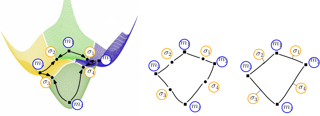
Himmelblau: (Compressed) Transition graph
(A) The landscape of Himmelblau, decomposed into the catchment basins of the four local minima (B) The transition graph, with one node for each critical (i.e., stationary) point (C) The compressed transition graph, where the information associated with saddles is stored in the edges joining local minima.

Prerequisites

We first recall the following two definitions (details def-transition-graph)):

A transition graph is a graph such that (i) nodes are local minima and saddle points, and (ii) an edge connects one local minimum and one saddle. A compressed transition graph is a graph in which the two edges emanating from a saddle have been merged.


The construction of the transition graph also output a weight for each local minimum. The weight is expected to code the probability of occupancy of the basin associated with the local minimum. Note that when persistence is used, the weight is the sum of the weights from the basins associated to the persistent local minimum.

Because weights are only on minima, we use the compressed transition graph representation, and set the weights on the vertices. There are two ways to set the weights:

TG built from a DB of stationary points. The weight of a local minimum is the normalized Boltzmann's factor computed using the energy of this local minimum. Beware of units for systems with reduced units, such as BLN69 for which both Boltzmann constant and temperature are set to unity. The following Python script computes the normalized Boltzmann's factor:

import sys, numpy
with open(sys.argv[1]) as fp: 
    exps = [numpy.exp(-float(l)) for l in fp]
    vals = [v/numpy.sum(exps) for v in exps]
    for v in vals: print(v)

TG built from sample points. The weight of a local minimum is the fraction of samples in the basin of the local minimum.

In that case, the user must specify energies only – since weights are computed from the fraction of samples in a basin.

Ideally, one may compute the weight of a basin by computing the partition function restricted to this basin. This task requires the calculation of density of states, which is beyond this application.


Applications from this package return of partition of the input into stable manifolds associated with local minima, see below. The two options just discussed (TG from sample points, TG from DB of critical points) call for one comment concerning the partition reported, which may or may not involve the stable manifold of saddle points. The reader is referred to section Graph connecting sample points versus graph connecting critical points for more details on these two options. Also check the –skip-saddle-SM option of the applications in this package.


Using sbl-tg-builder-lrmsd.exe from a database of stationary points

Pre-requisites

When a database of connected critical points (local minima and index one saddles) is available, building a transition graph is trivial.

We note that compressed transition graphs (rather than transition graphs) are built (definition def-compressed-tg), to minimize the memory footprint.

Main specifications

Main options.

The main options of the program sbl-tg-builder-lrmsd.exe are:
–from-DB: run transition graph building from a database
–discard-loops: remove from the transition graph all transitions incident to only one minimum
–points-file string(= plain text file listing all conformations as D-dimensional points (first for minima): second for transitions)
–energies string(= plain text file listing all energies (first for minima): second for transitions)
–weights string: plain text file listing weights on minima (e.g Boltzmann factors)
–samples-to-mins string: plain text file listing transitions as pairs of indices of minima


Two remarks are in order:
  • Points and energies are specified using the same option for both transitions and minima: the minima correspond always to the first specified file.
  • The samples-to-mins may appear as confusing since we do not map a sample to a min via quenching. Instead, when building a TG from a DB of stationary points, this option is used to provide the two indices of local minima connected via a saddle.


Input. The input consists of five files:

  • (txt format, suffix transitions.txt) Transition states: text file listing the pairs of minima linked by the transition states, on transition state per line
  • (Point_d format, suffix minima_conformations.txt) Local minima, geometry: text file listing the conformations of the local minima.
  • (txt format, suffix minima_energies.txt) Local minima, energy: text file listing the energies of the local minima.
  • (Point_d format, suffix transitions_conformations.txt) Transition states, geometry: text file listing the conformations of the TS.
  • (txt format, suffix suffix transitions_energies.txt) Transition states, energy: text file listing the energies of the TS.

Main output.

  • (txt format, suffix log.txt) Main log file.
  • (xml format, suffix tg.xml) Transition graph: output transition graph serialized into an XML archive.

Optional output.

Comments.

Using sbl-tg-builder-lrmsd.exe from a set of samples and associated local minima

Pre-requisites

Consider now the case where a plain sampling has been obtained, together with the local minimum associated with each sample (obtained by quenching) [165], [133] . Let us also assume that the transitions themselves have not been computed. In this case, one can locate pairs of conformations, say $(c_i, c_j)$ satisfying two conditions (see Fig. fig-morse-stable-unstable-manifolds-algo-flow-backward):

  • the conformations $c_i$ and $c_j$ are neighbor – their distance (for some suitable distance metric) is less than a user defined threshold;

  • the conformations $c_i$ and $c_j$ quench to different local minima.

Such a pairs is said to witness a bifurcation.
Note that the same two local minima may be witnessed by multiple pairs. For small enough value of the distance threshold, the sample with lowest energy amidst such pairs witnesses the adjacency of the catchment basins of $q(c_i)$ and $q(c_j)$. An algorithm to detect such pairs is sketched below, see section Algorithms and Methods.

Main specifications

Main options.

The main options of the program bl-tg-builder-lrmsd.exe are:
–from-sampling: run transition graph building from a sampling
–points-file string: plain text file listing all conformations or quenched conformations as D-dimensional points
–energies string: plain text file listing all energies of conformations or quenched conformations
–samples-to-mins string(= plain text file listing pairs of indices (conformations): quenched conformations)


Input.

  • (Point_d format, suffix conformations.txt) Conformations, geometry: a text file listing the conformations.
  • (txt format, suffix samples_energies.txt) Conformations, energies: energy of each conformation.
  • (Point_d format, suffix quenches_conformations.txt) Local minima, geometry: local minima obtained by quenching the conformations.
  • (txt format, suffix quenched_energies.txt) Quenched conformations, energies: text file with one energy of the local minima just described.
  • (txt format, suffix samples_to_quench.txt) Quench mapping: a file listing pairs of indices (conformation index, associated local min).

Main output.

  • (txt format, suffix log.txt) Main log file
  • (eps format, sufix , suffix disconnectivity_forest.eps) Disconnectivity forest in eps file format.
  • (xml format, suffix MSW_chain_complex.xml) Morse Smale Witten chain complex, which connects critical points in codimension one, serialized using Boost into an XML archive.
  • (xml format, suffix stable_manifold_partition.xml) Stable manifold partition: XML archive listing the samples repartition by persistent basin of the landscape.
  • (txt format, suffix persistence_diagram.txt) Persistence diagram, list of all basins sorted by persistence.
  • (txt format, suffix persistence_histogram.txt)
    Persistences: list of all finite persistences.
  • (pdf format, suffix persistence_histogram.pdf) Persistence histogram: pdf format, drawn by R.
  • (xml format, suffix wtg.xml) Transition graph: output transition graph serialized into an XML archive.

Optional output.

Comments.

Using sbl-tg-builder-euclid.exe from a set of samples

Pre-requisites

Consider finally the cases where only samples are known – that is the local minimum $q(c_i)$ associated with a conformation $c_i$ is unknown. Also assume that the neighborhood of $c_i$ has been densely sampled, and that $c_i$ has been connected to a set of nearest neighbors, using a nearest neighbor graph (NNG, definition def-nng). We estimate the gradient of the potential energy at $c_i$ using its neighbors in the NNG. More precisely, we estimate the gradient using the neighbor $c_k$ of $c_i$ yielding the maximum slope. Starting from $c_i$ and iteratively following this estimated gradient eventually leads to a sample having all its neighbors above it. One can use this sample as a substitute $\tilde{q}(c_i)$ for $q(c_i)$.

Main specifications

Main options.

The main options of the program bl-tg-builder-euclid.exe are:
–from-sampling: run transition graph building from a sampling
–points-file string: plain text file listing all conformations as D-dimensional points
–energies string: plain text file listing all energies
–persistence-threshold float: persistence threshold for removing not-persistent basins due to noisy data


Input.

  • (Point_d format, suffix conformations.txt) Conformations, geometry: a text file listing the conformations.
  • (txt format, suffix samples_energies.txt) Conformations, energies: energy of each conformation.
  • (real number) Persistence-threshold : threshold used to get rid of non persistent basins.

Main output.

  • (txt format, suffix log.txt) Main log file
  • (eps format, sufix , suffix disconnectivity_forest.eps) Disconnectivity forest in eps file format.
  • (xml format, suffix MSW_chain_complex.xml) Morse Smale Witten chain complex, which connects critical points in codimension one, serialized using Boost into an XML archive.
  • (xml format, suffix stable_manifold_partition.xml) Stable manifold partition: XML archive listing the samples repartition by persistent basin of the landscape.
  • (txt format, suffix persistence_diagram.txt) Persistence diagram, list of all basins sorted by persistence.
  • (txt format, suffix persistence_histogram.txt)
    Persistences: list of all finite persistences.
  • (pdf format, suffix persistence_histogram.pdf) Persistence histogram: pdf format, drawn by R.
  • (xml format, suffix wtg.xml) Transition graph: output transition graph serialized into an XML archive.

Optional output.

Comments.

Algorithms and Methods

In the following, we sketch the construction of the TG from a collection of points and associated local minima. The reader is also referred to the package Morse_theory_based_analyzer for further details (see also the MTBA module in the workflow, Fig. fig-tgb-workflow).

Assume that one is given a conformational ensemble $C$ together with the corresponding quenched points $C_q$. The algorithm consists of two main steps (Fig. fig-morse-stable-unstable-manifolds-algo-flow-backward):

  • Step 1: Nearest neighbor graph. We build a NNG on the conformations $C$ – see package Nearest_neighbors_graph_builder, and in addition endow each sample $c_i$ with an edge to $q(c_i)$. Note that this connection directly links each sample to its local minimum.

  • Step 2: Identification of transitions. Samples are sorted and processed by increasing energy. Upon inspecting a sample, we focus on its lower star, that is the subset of its neighbors with lower energy. We aim at identifying pairs of samples $(c_i,c_j)$, such that (i) $c_j$ belongs to the lower star of $c_i$ (recall that samples are processed by increasing height), and (ii) $q(c_i) \neq q(c_j)$. We also say that these samples witness a bifurcation. When such a pair of samples is found, we record the path from $q(c_i)$ to $q(c_j)$ through the samples $c_i$ and $c_j$. The collection of all such paths defines a transition graph between the vertices from the set $C_q$.
The following remarks are in order:
  • The bifurcations, as defined above, may involve more than two local minima. This is e.g. the case if a sample has in its lower star two or more samples flowing to distinct minima. This situation may occur in different settings: (i) in case of coarse sampling, the connected samples are located in the basins of several minima, (ii) the samples are located in the neighborhood of a critical point of index $>1$, or (iii) they are located in the neighborhood of a degenerate critical point (a so-called monkey saddle). Our method, which uses solely the samples, does not distinguish between these situations.
  • The saddles detected provide pessimistic estimates of barriers' heights. Also, they may not be close to the real saddles (i.e., critical points of index one of the PEL). The intuitive reason for this is that the stable manifold (catchment basin) of an index one saddle has dimension $d-1$ – the dimension of the whole configuration space minus one, which leaves ample space.
But they nevertheless indicate transitions between two basins associated with $q(c_i)$ and $q(c_j)$.


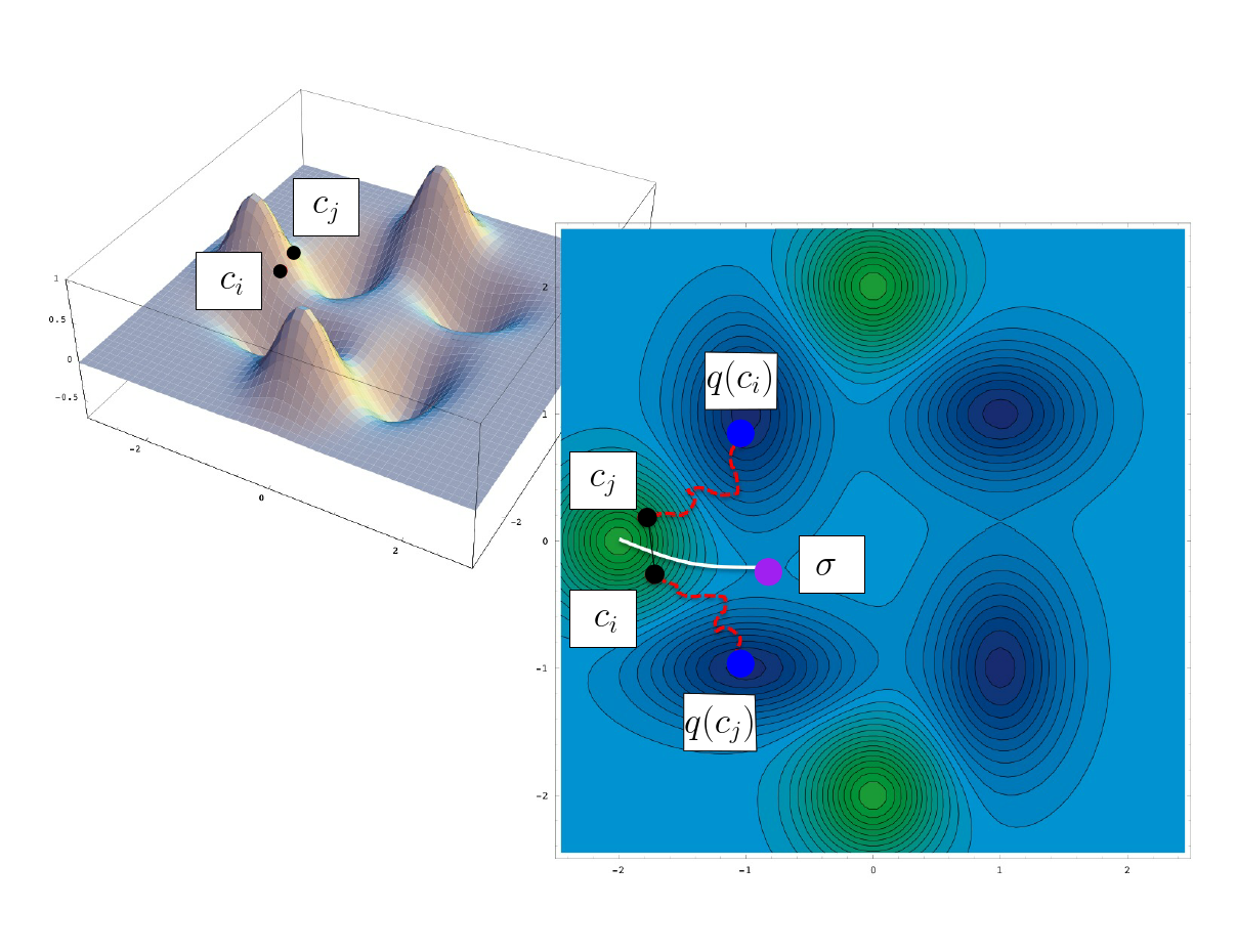
Identifying the connexion between the basins of two local minima by quenching two samples $c_i$ and $c_j$
Sample $c_i$ is quenched to $q(c_i)$ while $c_j$ is quenched to $q(c_j)$. The samples $c_i$ and $c_j$ sit across the (white) ridge separating the basins of their respective

Programmer's Workflow

The programs of Transition_graph_of_energy_landscape_builders described above are based upon generic C++ classes, so that additional versions can easily be developed.

In order to derive other versions, there are two important ingredients, that are the workflow class, and its traits class.

The Traits Class

T_Transition_graph_builder_from_sampled_energy_landscape_traits:

The Workflow Class

T_Transition_graph_builder_from_sampled_energy_landscape_workflow:

Other Utilities

For an analysis on the star of a vertex in a weighted graph, we recommand the use of the program sbl-energy-landscape-analysis-graph-star.exe, defined in the package Energy_landscape_analysis .

Jupyter demo

See the following jupyter notebook:

  • Jupyter notebook file
  • Transition_graph_of_energy_landscape_builders

    Transition_graph_of_energy_landscape_builders

    Useful functions

    In [1]:
    from SBL import SBL_pytools
    from SBL_pytools import SBL_pytools as sblpyt
    help(sblpyt)
     
    
    Help on class SBL_pytools in module SBL_pytools:
    
    class SBL_pytools(builtins.object)
     |  Static methods defined here:
     |  
     |  convert_eps_to_png(ifname, osize)
     |  
     |  convert_pdf_to_png(ifname, osize)
     |  
     |  find_and_convert(suffix, odir, osize)
     |      # find file with suffix, convert, and return image file
     |  
     |  find_and_show_images(suffix, odir, osize)
     |  
     |  find_file_in_output_directory(suffix, odir)
     |  
     |  show_eps_file(eps_file, osize)
     |  
     |  show_image(img)
     |  
     |  show_log_file(odir)
     |  
     |  show_pdf_file(pdf_file)
     |  
     |  show_row_n_images(images, size)
     |  
     |  show_text_file(file_suffix, odir)
     |  
     |  show_txt_file(file_suffix, odir)
     |  
     |  ----------------------------------------------------------------------
     |  Data descriptors defined here:
     |  
     |  __dict__
     |      dictionary for instance variables (if defined)
     |  
     |  __weakref__
     |      list of weak references to the object (if defined)
    
    
    In [ ]:


    Scenario 1: from a database of stationary points -- illustration on BLN conformations

    When a database of connected critical points (local minima and index one saddles) is available, building a transition graph is trivial.

    We note that compressed transition graphs (rather than transition graphs) are built, to minimize the memory footprint.

    Options

    The options of the runFromDatabase method in the next cell are:

    • metric: euclid or lrmsd
    • discardLoop: remove from the transition graph all transitions incident to only one minimum
    • minimaPoints: plain text file listing all minima conformations as D-dimensional points
    • transitionPoints: plain text file listing all transition conformations as D-dimensional points
    • minimaEnergies: plain text file listing all minima energies
    • transitionEnergies: plain text file listing all transition energies
    • samples2Mins: plain text file listing transitions as pairs of indices of minima
    • weights: optional plain text file listing minima weights for a weighted transition graph

      Nb: by default, no persistence is used. But the executable used can also use persistence.

    In [4]:
    from SBL import TG_builders
    from TG_builders import *
    
    
    sbl_exe_name = "sbl-tg-builder-lrmsd.exe"
    odir= "tmp-results-db-lrmsd"
    tg1 = TG_builders.build_transition_graph_fromDB(sbl_exe_name,
                                        "data/bln69_database_minima_conformations.txt",  "data/bln69_database_minima_energies.txt",
                                        "data/bln69_database_transitions_conformations.txt",  "data/bln69_database_transitions_energies.txt",
                                        "data/bln69_database_transitions.txt",
                                        odir,
                                        "data/bln69_database_minima_weights.txt")
    print(tg1)
    sblpyt.list_directory_content(odir)
    
    Executing /user/fcazals/home/projects/proj-soft/sbl-install/bin/sbl-tg-builder-lrmsd.exe --from-DB --samples-to-mins data/bln69_database_transitions.txt                 --points-file data/bln69_database_minima_conformations.txt --energies data/bln69_database_minima_energies.txt --points-file data/bln69_database_transitions_conformations.txt --energies data/bln69_database_transitions_energies.txt                 --directory tmp-results-db-lrmsd --verbose --log --discard-loops --weights data/bln69_database_minima_weights.txt
    
    tmp-results-db-lrmsd/sbl-tg-builder-lrmsd__tg.xml
    Files in directory tmp-results-db-lrmsd: ['sbl-tg-builder-lrmsd__log.txt\n', 'sbl-tg-builder-lrmsd__tg.xml\n']
    
    In [ ]:
     
    
    In [ ]:


    Scenario 2: from a set of samples and associated local minima -- illustration on BLN conformations

    Consider now the case where a plain sampling has been obtained, together with the local minimum associated with each sample (obtained by quenching). Let us also assume that the transitions themselves have not been computed. In this case, one can locate pairs of conformations, say $(c_i, c_j)$ satisfying two conditions:

    • the conformations $c_i$ and $c_j$ are neighbor – their distance (for some suitable distance metric) is less than a user defined threshold;

    • the conformations $c_i$ and $c_j$ quench to different local minima.

    Such a pairs is said to witness a bifurcation. Note that the same two local minima may be witnessed by multiple pairs. For small enough value of the distance threshold, the sample with lowest energy amidst such pairs witnesses the adjacency of the catchment basins of $q(c_i)$ and $q(c_j)$.

    Options

    The options of the runFromMinima method in the next cell are:

    • metric: euclid or lrmsd
    • conformationPoints: plain text file listing all conformations as D-dimensional points
    • conformationEnergies: plain text file listing all conformation energies
    • quenchedPoints: plain text file listing all quenched conformations as D-dimensional points
    • quenchedEnergies: plain text file listing all quenched conformation energies
    • samples2Mins: plain text file listing pairs of indices (conformations, quenched conformations)

    Nb: by default, no persistence is used. But the executable used can also use persistence.

    In [5]:
    from SBL import TG_builders
    from TG_builders import *
    
    sbl_exe_name = "sbl-tg-builder-lrmsd.exe"
    odir= "tmp-results-quench-lrmsd"
    tg = TG_builders.build_transition_graph_from_minima(sbl_exe_name,
                                                        "data/bln69_sampling_samples_conformations.txt", "data/bln69_sampling_samples_energies.txt",
                                                        "data/bln69_sampling_quenched_conformations.txt", "data/bln69_sampling_quenched_energies.txt",
                                                        "data/bln69_sampling_samples_to_quench.txt", odir)
    print(tg)
    sblpyt.list_directory_content(odir)
    
    /user/fcazals/home/projects/proj-soft/sbl-install/bin/sbl-tg-builder-lrmsd.exe
    Executing /user/fcazals/home/projects/proj-soft/sbl-install/bin/sbl-tg-builder-lrmsd.exe --from-sampling                   --points-file data/bln69_sampling_samples_conformations.txt --energies data/bln69_sampling_samples_energies.txt --points-file data/bln69_sampling_quenched_conformations.txt --energies data/bln69_sampling_quenched_energies.txt --samples-to-mins data/bln69_sampling_samples_to_quench.txt                   --directory tmp-results-quench-lrmsd --verbose --log --num-neighbors 8
    
    tmp-results-quench-lrmsd/sbl-tg-builder-lrmsd__wtg.xml
    Files in directory tmp-results-quench-lrmsd: ['sbl-tg-builder-lrmsd__disconnectivity_forest.eps\n', 'sbl-tg-builder-lrmsd__log.txt\n', 'sbl-tg-builder-lrmsd__MSW_chain_complex.xml\n', 'sbl-tg-builder-lrmsd__nng.xml\n', 'sbl-tg-builder-lrmsd__persistence_diagram.pdf\n', 'sbl-tg-builder-lrmsd__persistence_diagram.plot\n', 'sbl-tg-builder-lrmsd__persistence_diagram.txt\n', 'sbl-tg-builder-lrmsd__persistence_histogram.pdf\n', 'sbl-tg-builder-lrmsd__persistence_histogram.r\n', 'sbl-tg-builder-lrmsd__persistence_histogram.txt\n', 'sbl-tg-builder-lrmsd__stable_manifold_clusters.txt\n', 'sbl-tg-builder-lrmsd__stable_manifold_partition.xml\n', 'sbl-tg-builder-lrmsd__wtg.xml\n']
    

    Let us visualize the disconnectivity tree and the persistence diagram

    In [6]:
    odir = "tmp-results-quench-lrmsd"
    images = []
    images.append( sblpyt.find_and_convert("disconnectivity_forest.eps", odir, 100) )
    images.append( sblpyt.find_and_convert("persistence_diagram.pdf", odir,100) )
    sblpyt.show_row_n_images(images, 100)
    
    Figs displayed
    
    In [ ]:


    Scenario 3 : from a set of samples -- illustration on the 2D terrain Himmelblau

    Consider finally the cases where only samples are known – that is the local minimum $q(c_i)$ associated with a conformation $c_i$ is unknown. Also assume that the neighborhood of $c_i$ has been densely sampled, and that $c_i$ has been connected to a set of nearest neighbors, using a nearest neighbor graph (NNG). We estimate the gradient of the potential energy at $c_i$ using its neighbors in the NNG. More precisely, we estimate the gradient using the neighbor $c_k$ of $c_i$ yielding the maximum slope. Starting from $c_i$ and iteratively following this estimated gradient eventually leads to a sample having all its neighbors above it. One can use this sample as a substitute $\tilde{q}(c_i)$ for $q(c_i)$.

    Options

    The options of the runFromSamples method in the next cell are:

    • metric: euclid or lrmsd
    • conformationPoints: plain text file listing all conformations as D-dimensional points
    • conformationEnergies: plain text file listing all conformation energies
    • persistence: ersistence threshold for removing not-persistent basins due to noisy data

      Nb: by default, no persistence is used. But the executable used can also use persistence.

    In [ ]:
     
    
    In [7]:
    from SBL import TG_builders
    from TG_builders import *
    
    sbl_exe_name = "sbl-tg-builder-euclid.exe"
    odir = "tmp-results-sampling"
    
    tg = TG_builders.build_transition_graph_from_sampling(sbl_exe_name, "data/himmelblau_rand_points.txt", "data/himmelblau_rand_heights.txt", odir)
    print(tg)
    sblpyt.list_directory_content(odir)
    
    /user/fcazals/home/projects/proj-soft/sbl-install/bin/sbl-tg-builder-euclid.exe
    Executing /user/fcazals/home/projects/proj-soft/sbl-install/bin/sbl-tg-builder-euclid.exe --from-sampling         --points-file data/himmelblau_rand_points.txt --energies data/himmelblau_rand_heights.txt --persistence-threshold -1.000000               --directory tmp-results-sampling --verbose --log --num-neighbors 8
    
    tmp-results-sampling/sbl-tg-builder-euclid__wtg.xml
    Files in directory tmp-results-sampling: ['sbl-tg-builder-euclid__disconnectivity_forest.eps\n', 'sbl-tg-builder-euclid__log.txt\n', 'sbl-tg-builder-euclid__MSW_chain_complex.xml\n', 'sbl-tg-builder-euclid__nng.xml\n', 'sbl-tg-builder-euclid__persistence_diagram.pdf\n', 'sbl-tg-builder-euclid__persistence_diagram.plot\n', 'sbl-tg-builder-euclid__persistence_diagram.txt\n', 'sbl-tg-builder-euclid__persistence_histogram.pdf\n', 'sbl-tg-builder-euclid__persistence_histogram.r\n', 'sbl-tg-builder-euclid__persistence_histogram.txt\n', 'sbl-tg-builder-euclid__stable_manifold_clusters.txt\n', 'sbl-tg-builder-euclid__stable_manifold_partition.xml\n', 'sbl-tg-builder-euclid__wtg.xml\n']
    
    In [8]:
    odir = "tmp-results-sampling"
    images = []
    images.append( sblpyt.find_and_convert("disconnectivity_forest.eps", odir, 100) )
    images.append( sblpyt.find_and_convert("persistence_diagram.pdf", odir,100) )
    sblpyt.show_row_n_images(images, 100)
    
    Figs displayed
    
    In [ ]:
     
    
    In [ ]:
     
    
    In [ ]:
     
    
    In [ ]: