Structural_motifs

Authors: F. Cazals and R. Tetley

Introduction

Structural motifs. Structural alignment methods for polypeptide chains aim at identifying conserved structural motifs between structures.

Global structural alignment methods often fail to exploit local properties, i.e. locally conserved distances. Phrased differently, for similarity measures such as $\lrmsd$ (see Molecular_distances and Molecular_distances_flexible), large values between two structures possibly obliterates regions of smaller size and with a much better structural conservation.

This package provides a method identifying locally conserved hierarchical structural motifs shared by two polypeptide chains whose structure is known. In a nutshell:

A structural motif consists in two sets of a.a., one on each structure, such that the $\lrmsd$ of the motif is significantly smaller than that associated with a global alignment between the two structures: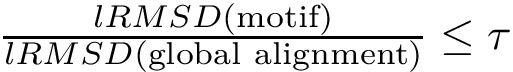

For each structure, all the motifs reported form a partially ordered set, which can be represented using a directed acyclic graph (or Hasse diagram).

$\lRMSDRatio \leq \tau$

Applications involving structural motifs. Motifs may be used to compute combined $\rmsd$ as done in Molecular_distances_flexible , and/or investigate the homology between proteins using profile hidden Markov models as done in FunChaT .

Prerequisites

In the sequel, we recall the main concepts and the four steps used to identify motifs, referring the reader to [41] for the details.

For the sake of conciseness, we use structure and polypeptide chain interchangeably; likewise, structural motif and motif are used interchangeably.

Step 1: Computing the seed alignment and its scores

Consider two polypeptide chains and of length and . Also consider a seed alignment between them; let $N \leq \min(n_A, n_B)$ be its length, namely the number of a.a. matched.

The alignment consists of pairs of a.a. mapped with one another, and can be computed using various methods. In this package, we use the following two aligners:

$\text{\apurva}$ is a structural aligner based on contact maps, favoring long and flexible alignments [11]. See the package Apurva .

$\text{\kpax}$ is a structural aligner based on a geometric representation of the backbone, favoring a geometric measure known as the G-score [151]. See the package Iterative_alignment .

Denoting $\distaij$ the distance between the $\Calpha$ carbons of indices i and j on chain , and likewise on chain , an assessment of the matching is provided by the distance difference matrix (DDM), a $N \times N$ symmetric matrix whose entries, also called scores, are given by:

$\scoreij = \fabs{\distaij - \distbij}, i = 1, \dots, N, j=1, \dots, N$

Note that these distances qualify the conservation of distances between $\Calpha$ between the two structures.

Step 2: Building the filtration and its space filling diagram

In mathematics, a filtration is a (finite) sequence of nested spaces [79] . Our method uses a filtration which may be the conserved distances (CD) filtration or the space filling diagram (SFD) filtration.

Conserved distances (CD) filtration. For each molecule, consider a graph whose vertices represent a.a., and edges are associated with all pairs of a.a (complete graph). Each edge is weighted by the score $\scoreij$ . Assume that edges have been sorted in ascending order.

To each edge weight–say , corresponds a graph containing only those edges whose weight is $\leq w$ . In processing edges by increasing value, these graphs are nested. We call this sequence of graphs the conserved distances (CD) filtration.

Space filling diagram (SFD) filtration. Molecular models defined by union of balls are called space filling diagrams (SFD). Geometric and topological properties of such diagrams are encoded in the so-called $\alpha$ -complex (see Alpha_complex_of_molecular_model , as well as Space_filling_model_surface_volume ).

Upon sorting the scores $\scoreij$ by ascending value, define the absolute $\Calpha$ rank of a given a.a. as the smallest index of a score involving that $\Calpha$ . Finally, let the $\Calpha$ rank of a given a.a. be the index of its absolute $\Calpha$ rank (see details in [41] ).

For each molecule, to each index–say , corresponds a SFD containing only those a.a. whose index is $\leq i$ . In processing indices by increasing value, these SFD are nested. We call this sequence of SFD the SFD filtration.

Persistence diagram. For either filtration, let us focus on connected components, which appear and disappear when inserting edges (CD filtration) or a.a. (SFD filtration). A union-find data structure can be used to maintain these c.c. [61], and track in particular the birth date and the death date of each component.

The collection of all these points ${(\text{birth date}, \text{death date})}$ defines a 2D diagram called the persistence diagram [79] . Note that all points lie above the diagonal ; moreover, the distance of a point to the diagonal is the lifetime of the c.c. associated to that point.

To compute persistence diagrams, we use the Morse_theory_based_analyzer package.

Step 3: Computing structural motifs

As previously stated, for each structure we compute a persistence diagram, respectively denoted $\persDiagA$ and $\persDiagB$ .

Two points located in the same region of their respective PD have comparable birth and death dates. We identify such pairs of points. Denote $a \in \persDiagA$ and $b\in \persDiagB$ two such points. We say that and are comparable if the Euclidean distance between the two points (computed by using their respective birth and death dates as coordinates) is below a given threshold $\tau_{PD}$ .

When two points are comparable, we identify motifs as follows:

First, we compute the connected components associated to the sublevel set of the graph (CD filtration), or SFD (SFD filtration).
Second, we perform a structural alignment between all pairs of connected components. We distinguish the cases of homologous proteins and that of conformations:
- Homologous proteins: the aligner used is that used to compute the seed alignment.
- Conformations: the sequences being identical, the alignment is trivial. To enlarge the size of motifs, we perform a one step clustering of c.c. using the D-family matching algorithm from D_family_matching. In a nutshell, this method finds a many-to-many correspondence between connected components.
Third, we selected the alignments satisfying the $\text{\lrmsd}$ ratio of Eq. eq-lrmsdratio .

Practically, we impose constraints on motifs:

comparable points in PD: we impose a distance between points of at most $\tau_{PD} (= 20)$
size constraint: a motif should contain at least a.a.
$\text{\lrmsd}$ ratio: should be at most $\tau (= 0.7)$

Note that for a given structure, a structural motif is not necessarily connected, neither on the structure, nor on the sequence. This stems from the fact that a motif is defined upon performing a structural alignment on two connected components (from sublevel sets of the CD or SFD filtration). In practice, though, motifs are generally connected on the structure, but not on the sequence. See details in the companion paper [41] .

Step 4: Filtering structural motifs

As detailed in [41] , motifs are filtered in two ways:

Motif inclusion. A Hasse diagram is used to detect the nestedness of motifs. The Hasse diagram is defined from the partial order induced by the inclusion between sets of a.a. defining structural motifs.

Statistical significance. The statistical significance of motifs is obtained via a two-sample-test p-value calculation (Wilcoxon Mann-Whitney), comparing the motifs obtained against random motifs.

Bonus steps: combined RMSD and seeding iterative alignment

As detailed in [41], motifs can be used to compute the edge-weighted $\text{\rmsdcomb}$ (see Molecular_distances_flexible). Additionally, structural motifs can be used to seed an iterative aligner (see the package Iterative_alignment).

Using structural motif finders

Programs

As explained above, the detection of motifs hinges on two ingredients:

An initial seed alignment. To handle two different proteins, we use two seed aligners ( $\text{\apurva}$ , $\text{\kpax}$ ). To handle two conformations of the same protein, the trivial identity alignment is used.

A filtration. We use two options: the filtration of conserved distances (CD), and the filtration based on space filling diagrams (SFD).

Combining these yields four methods:

Aligners requiring an alignment: $\text{\alignerkpaxcd}$ , $\text{\alignerkpaxsfd}$ , $\text{\alignerapurvacd}$ , $\text{\alignerapurvasfd}$ .

Aligners with the identity alignment: $\text{\aligneridcd}$ , $\text{\aligneridsfd}$ .

These four methods are implemented within the following executables: each giving access to the CD and SFD filtrations:

$\text{\sblsmotifsapurva}$ : structural motifs for proteins, using the $\text{\apurva}$ aligner
$\text{\sblsmotifskpax}$ : structural motifs for proteins, using the $\text{\kpax}$ aligner
$\text{\sblsmotifsconf}$ : structural motifs for conformations

By default, all the executables search for structural motifs which are then used to compute the $\text{\rmsdcomb}$ and seed an iterative alignment. The results of these two bonus calculations are always output.

Main specifications

We illustrate how to run the program on one executable since all behave in the same manner.

Input. In a nutshell:

A pair of proteins, in PDB file format.

Possibly a specification of domains for these proteins. This enables searching for motifs in nested regions of the protein. The specification file is a simpler version of the one described in MolecularSystemLabelsTraits : one line per domain containing in sequential order the domain name, the number of residue ranges and the residue sequence number ranges (examples below).

Main options. The main options are:

–pdb-file string: PDB file passed twice ie once for each structure
–chains string: Chain(s) to load passed twice ie once for each structure
–allow-incomplete-chains: Allow loading incomplete structures
–motif-size: The motif size threshold

–lrmsd-threshold: The $\text{\lrmsd}$ threshold $\tau$
–load-domains: The domains spec file. Domains are defined as residue sequence number ranges.

If no domains are specified using the –load-domains option, the executable searches for a file with the same prefix as the PDB file but with the .dom extension in the PDB file directory.

Main output. As stated in Introduction, we report motifs for each structure. Each motif is identified by a unique motif id .

The main files output are as follows:

Motifs file, xml file, suffix __persistent_motifs.xml : XML Archive of all the found structural motifs. The archive provides two pieces of information. First, one finds statistics on the global alignment between the two chains. Second next, one finds the following pieces of information for every structural motif:
- motif index (tag motif_index)
- motif size (alignment_size)
- motif persistence (first_motif_persistence, second_motif_persistence)
- motif lRMSD and dRMSD (tags lrmsd and drmsd)
- residues involved in the motif (tags first_motif_resids, second_motif_resids).
Nb: the python module Structural_motifs defines classes to parse this file and retrive the information on motifs. See also the script sbl-structural-motifs-analyzer.py, described below.

serialization seen in the file *persistent_motifs.xml done by class SBL::Modules::T_Pairwise_structural_alignment_module from file Pairwise_structural_alignment_module.hpp
Motifs diagram, GraphViz file, suffix hasse_diagram_one.dot: Hasse diagram of motifs. Each motif is identified with a unique index.
(todo) Motifs graph, xml file, suffix motif_graph.xml: XML Archive of the so-called motif graph (see Molecular_distances_flexible)
Pymol scripts, python file, suffix .py: one script for each structural motif, as discussed below.

Additional files of interest are:

Log file (if option –log used), suffix log.txt: main log file.
Alignment file, txt file, suffix __alignment.txt : the initial alignment, for re-running purposes.

Example one: motifs for conformations

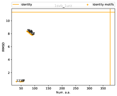
As a first example, we illustrate the conformational change undergone a prototypical class II fusion protein, from the tick-borne encephalitis virus. The ectodomain of this protein was crystallized both in soluble form (PDB: 1SVB, 395 residues) and in postfusion conformation (PDB: 1URZ, 401 residues).

For these structures, the identity alignment identifies 376 a.a., with a reference lRMSD of 1.13 – see yellow lines on Fig. fig-rigid-blocks-confs .

We run the executable as follows:

./sbl-structural-motifs-conformations.exe  --motif-size 30 --lrmsd-threshold 0.8 --allow-incomplete-chains -p 4 --pdb-file pdb/1svb.pdb --chains A --pdb-file pdb/1urz.pdb --chains A --log -d 1svb-1urz

and generate the plots with

sbl-structural-motifs-analyzer.py -d 1svb-1urz

Rigid blocks for 1n75/chain A vs 3afh/chain A: size (number of a.a.) versus lRMSD

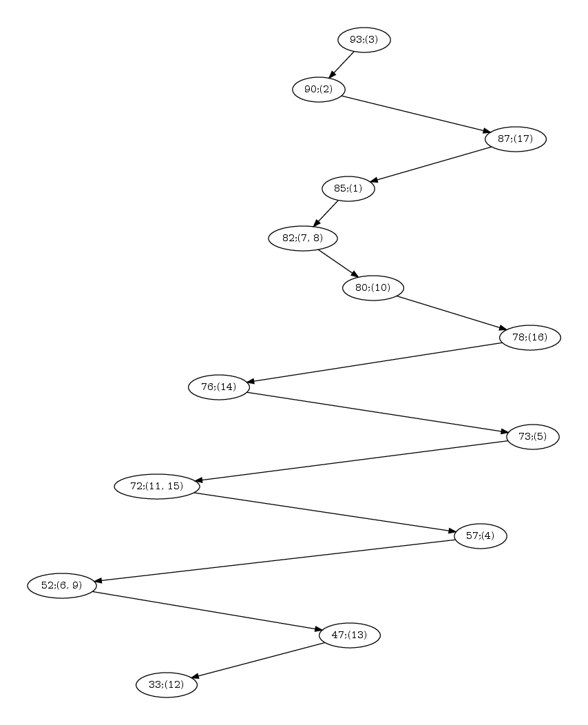Hasse diagram for the nested-ness of domains in the comparison 1svb vs 1urz. The labels x; (y,z) in a node read as follows: x is the number of residues in the motif; (y,z) are the motif indices, as reported in the persistent_motifs.xml xml file. An arrow between two motifs indicates the inclusion for the corresponding amino acid sets.

The following comments are in order:

Scatter plot. Fig. fig-rigid-blocks-confs

Hasse diagram. Fig. fig-hasse-confs

Example two: motifs for homologous chains

As a second illustration, we compare two proteins 1n75 (chain A, 468 residues) and 3afh (chain A, 488 residues).

For these structures, the reference alignment involves 431 a.a., for a lRMSD of 2.05 – yellow lines on Fig. fig-rigid-blocks-chains .

sbl-structural-motifs-chains-kpax.exe  --motif-size 30 --lrmsd-threshold 0.8 --allow-incomplete-chains -p 4 --pdb-file pdb/1n75.pdb --chains A --pdb-file pdb/3afh.pdb --chains A --log -d 1n75-3afh

and generate the plots with

sbl-structural-motifs-analyzer.py -d 1n75-3afh

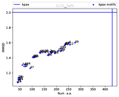Rigid blocks for 1n75/chain A vs 3afh/chain A: size (number of a.a.) versus lRMSD

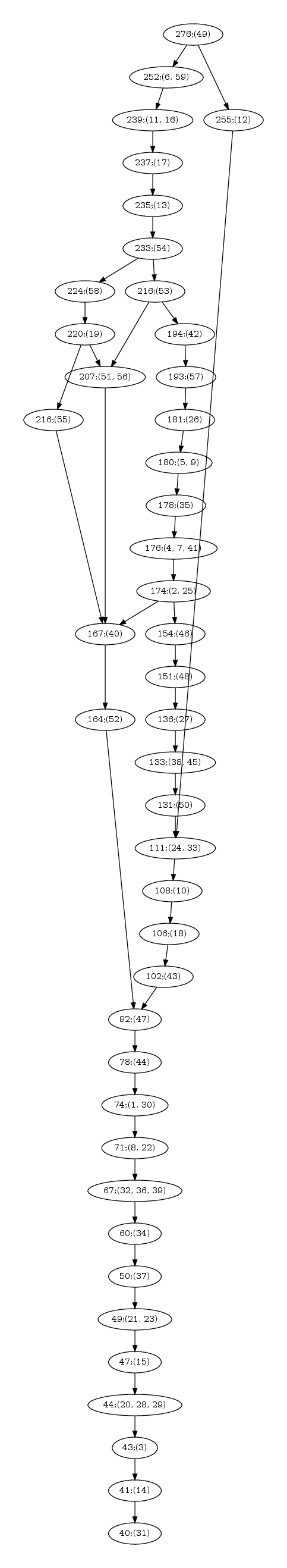Hasse diagram for the nested-ness of domains in the comparison of 1n75 vs 3afh. The labels x; (y,z) in a node read as follows: x is the number of residues in the motif; (y,z) are the motif indices, as reported in the persistent_motifs.xml xml file. An arrow between two motifs indicates the inclusion for the corresponding amino acid sets.

Scatter plot.

Fig. fig-rigid-blocks-chains

Hasse diagram. Fig. fig-hasse-chains

Using the PyMol scripts

To further investigate each structural motif, the executable outputs PyMol scripts. In order to run the script corresponding to, say motif 8, in the previous run, the user should follow these steps:

Open PyMol

Load each of the structures. In PyMol:

load data/1URZ.pdb
load data/1SVB.pdb

Run the script corresponding to said motif. In PyMol:

run results/conformations-sf/sbl-structural-motifs-conformations__block_8_script.py

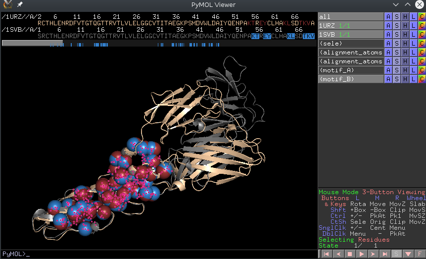A screenshot of the PyMol window after running one of the outputted pymol scripts

PyMol scripts for viewing the final iterative alignment are also outputted (sbl-structural-motifs-conformations__iterative_alignment.py).

Using the VMD script

To be developed.

Using python scripts

The package provides two python scripts:

sbl-structural-motifs-computer.py.

Consider a list of four-tuples, namely {(pdbid1, chain1, pdbid2, chain2)}, listed in a text file. The following call uses $\text{\sblsmotifskpax}$ and/or $\text{\sblsmotifsapurva}$ (see option -a) to perform a motif calculation for each four-tuple:

sbl-structural-motifs-computer.py -i fatcat2003 -f fatcat2003/fatcat2003--small.txt -a three

sbl-structural-motifs-analyzer.py.

The scatter plots for motifs indicate motif ids, and the associated Hasse diagram (one for each molecule) also indicates how motifs are nested. The following script processes a directory generated by the previous script, and proposes two analysis:

If one motif index is given: the list of resids in this motif is printed.

If two motif indices are given, the symmetric difference between the corresponding lists of resids is printed. This analysis eases the interpretation of Hasse diagrams.

The following call lists the resids found in the motif whose id is 5:

dulfer-fcazals> ./sbl-structural-motifs-analyzer.py -d results/apurva/1CID.pdb-A--2RHE.pdb-A -m 5
Motif file is results/apurva/1CID.pdb-A--2RHE.pdb-A/sbl-structural-motifs-chains-apurva__persistent_motifs.xml
Log file is results/apurva/1CID.pdb-A--2RHE.pdb-A/sbl-structural-motifs-chains-apurva__log.txt
Initial alignment size: 103.0
Initial alignment lRMSD: 3.944686
XML: 1 / 1 files were loaded

('Motif indices:', [1, 2, 3, 4, 5, 7, 8, 10, 11, 12, 13, 14, 15, 16, 17, 18])
('Motif lrmsds:', [1.715135302837146, 3.027206911843852, 2.794978851169716, 3.03162145728718, 1.4790716539949267, 1.7351701619296112, 1.695979267778361, 2.9667660204140045, 3.0269885774433014, 2.689248812159066, 3.031806753459111, 2.739264842927472, 1.6532866267424344, 2.871028387233174, 3.031927685048948, 3.0744944632903914])
('Motif sizes:', [34, 77, 47, 63, 12, 17, 19, 40, 68, 52, 75, 50, 32, 44, 66, 61])

List of the 12 resids in molecule 1 for motif index 5:
[9, 10, 13, 16, 26, 31, 73, 83, 95, 96, 97, 98]
12 resids in molecule 2 for motif index 5:
[14, 15, 18, 21, 32, 37, 73, 83, 97, 98, 99, 100]
dulfer-fcazals>

The following call compares the lists of resids associated with two motif ids – which is especially useful to investigate the relationship between motifs of interest identified on the Hasse diagram of motifs:

dulfer-fcazals> ./sbl-structural-motifs-analyzer.py -d results/apurva/1CID.pdb-A--2RHE.pdb-A -m 5 -n 7
Motif file is results/apurva/1CID.pdb-A--2RHE.pdb-A/sbl-structural-motifs-chains-apurva__persistent_motifs.xml
Log file is results/apurva/1CID.pdb-A--2RHE.pdb-A/sbl-structural-motifs-chains-apurva__log.txt
Initial alignment size: 103.0
Initial alignment lRMSD: 3.944686
XML: 1 / 1 files were loaded

('Motif indices:', [1, 2, 3, 4, 5, 7, 8, 10, 11, 12, 13, 14, 15, 16, 17, 18])
('Motif lrmsds:', [1.715135302837146, 3.027206911843852, 2.794978851169716, 3.03162145728718, 1.4790716539949267, 1.7351701619296112, 1.695979267778361, 2.9667660204140045, 3.0269885774433014, 2.689248812159066, 3.031806753459111, 2.739264842927472, 1.6532866267424344, 2.871028387233174, 3.031927685048948, 3.0744944632903914])
('Motif sizes:', [34, 77, 47, 63, 12, 17, 19, 40, 68, 52, 75, 50, 32, 44, 66, 61])

List of the 12 resids in molecule 1 for motif index 5:
[9, 10, 13, 16, 26, 31, 73, 83, 95, 96, 97, 98]
12 resids in molecule 2 for motif index 5:
[14, 15, 18, 21, 32, 37, 73, 83, 97, 98, 99, 100]

List of the 17 resids in molecule 1 for motif index 7:
[9, 10, 13, 16, 25, 26, 28, 31, 60, 67, 73, 83, 84, 95, 96, 97, 98]
17 resids in molecule 2 for motif index 7:
[14, 15, 18, 21, 31, 32, 34, 37, 59, 66, 73, 83, 84, 97, 98, 99, 100]

[molecule1] Symmetric differences, sizes 0 12 5

Symmetric differences, items:
('A minus B:', [])
('A intersection B:', [9, 10, 13, 16, 26, 31, 73, 83, 95, 96, 97, 98])
('B minus A', [25, 28, 60, 67, 84])

[molecule2] Symmetric differences, sizes 0 12 5

Symmetric differences, items:
('A minus B:', [])
('A intersection B:', [14, 15, 18, 21, 32, 37, 73, 83, 97, 98, 99, 100])
('B minus A', [31, 34, 59, 66, 84])

Implementation and functionalities

The implementation is straight-forward: each step described in the previous section is computed in a module, which are all linked together in the following workflow.

Main classes

The package Structural_motifs uses two novel data structures, the filtration graphs. These were implemented in the classes:

SBL::CSB::T_Filtration_graph_SFD< Structure , AlphaComplex >. Given an input structure, it builds a vertex weighted graph. This graph corresponds to the history of contacts between residues upon inserting them in a given order. The order is associated with a filtration function, in our case the $\Calpha$ ranks. The first template parameter is the representation of a proteic structure. It should contain residues which provide access to their $\Calpha$ ranks as well as to their usual information. The second parameter is an alpha complex. Practically, we use the class defined in Alpha_complex_of_molecular_model.

SBL::CSB::T_Filtration_graph_CD< Structure >. Given an input structure, it builds an edge weighted graph. The vertices are the set of residues, and the edges correspond to all pairs of a.a. (complete graph). The edge weights correspond to the order in which a residue pair appears in the ordering of $s_{ij}$ scores. The template parameter is the representation of a proteic structure. .

These two classes allow to switch between the different types of filtration.

Modules

The package Structural_motifs is centered around two main new modules:

SBL::Modules::T_Pairwise_structural_alignment_module< ModuleTraits > inherits from SBL::Modules::T_Alignment_structures_module< ModuleTraits >. This module has two run modes. In the first mode, it computes a structural alignment between the two input structures and the $s_{ij}$ ordering. In the second mode, it simply computes an alignment and a $\lrmsd$ . This is necessary for step 4.

SBL::Modules::T_Filtration_graph_module< ModuleTraits > is the module associated with the previously defined classes. It is used for step 2 of the computation.

The package also uses the following modules:

From the weighted graph built by SBL::Modules::T_Filtration_graph_module< ModuleTraits > one can compute the persistence diagram of connected components. This is done by using SBL::Modules::T_Morse_theory_based_analyzer_for_vertex_weighted_graph_module< ModuleTraits >. For more details see Morse_theory_based_analyzer. It is used for step 3 of the computation.

SBL::Modules::T_RMSD_comb_edge_weighted_module< ModuleTraits > is used to compute the $\text{\rmsdcomb}$ from the list of structural motifs found in the previous steps.

SBL::Modules::T_Iterative_alignment_module< ModuleTraits > is used to seed an iterative aligner with the previously computed structural motifs.

SBL::Modules::T_Iterative_alignment_module< ModuleTraits > was created as a new module in this package because it goes beyond the use cases of the module in Iterative_alignment.

T_Structural_motifs_workflow:

Jupyter demo

See the following jupyter notebook:

Jupyter notebook file
Structural_motifs
Structural_motifs¶
Recall that the SBL provides three executables to mine motifs shared by two structures:

sbl-structural-motifs-conformations.exe

sbl-structural-motifs-chains-apurva.exe and sbl-structural-motifs-chains-kpax.exe , which use two different methods for seed alignments, namely Apurva and Kpax.

The main difference is that for conformations of the same molecule, we do not need to compute any alignment.

In the sequel, we focus on conformations -- using the remaining two executables is similar.
Useful general functions¶

Case study I: extracting motifs using Conserved Distances (CD) filtration¶

Run the calculation¶
In [1]:

from SBL import Structural_motifs from Structural_motifs import * from SBL import SBL_pytools from SBL_pytools import SBL_pytools as sblpyt #help(sblpyt) # Structural motifs general options smgo = Structural_motifs_general_options() smgo.update_mode("conformations") print("General options are: ", str(smgo)) # Prepare the 4-tuple to be processed smgo.set("input_dir", "fusion-class-II") data = ("1SVB.pdb", "A", "1URZ.pdb", "A") # Create an instance of the algo and run it sm_for_pairs = Structural_motifs_computer_for_pair(smgo) res_triple = sm_for_pairs.process_two_structures( data ) res_triple.dump()
General options are: {'input_dir': '', 'input_list': '', 'occupancy': 4, 'mode': 'conformations', 'use_sfd': False, 'min_motif_size': 10, 'lrmsd_ratio': 0.8, 'pd_dist_threshold': 0.8, 'show_diagrams': False, 'odir_root': 'results', 'verbose': False, 'dry': False, 'aligner': 'identity', 'exe': '/user/fcazals/home/projects/proj-soft/sbl-install/bin/sbl-structural-motifs-conformations.exe'} /user/fcazals/home/projects/proj-soft/sbl-install/bin/sbl-structural-motifs-conformations.exe --motif-size 10 --lrmsd-threshold 0.8 --allow-incomplete-chains -p 4 --pdb-file fusion-class-II/1SVB.pdb --chains A --pdb-file fusion-class-II/1URZ.pdb --chains A --directory-output results/identity-cd/1SVB-A--1URZ-A --module-uid --log Log file: results/identity-cd/1SVB-A--1URZ-A/sbl-structural-motifs-conformations__log.txt Res-triple: Aligner: identity Concatenation of pdb ids: 1SVB-1URZ Output directory: results/identity-cd/1SVB-A--1URZ-A
Collect statistics and perform the plots¶

Socre plot. Recall that the C-alpha ranks are obtained from a structural distance score, namely the distance difference between two C-alpha carbons. If CA_i and CA_j are aligned to CA_i' and CA_j' respectively, the distance difference is s_ij = |d_ij - d_i'j'| where d_ij = |CA_i - CA_j|. We can plot the s_ij scores against their respective C-alpha ranks.

Calpha distance plot. For a given C-alpha rank we can recover the corresponding C-alpha carbons CA_i and CA_j. We can then plot |CA_i - CA_j| (or |CA_i' - CA_j'| for the second structure) against the C-alpha rank. This gives us an indication on how the atoms are selected on the structure. Notice the distinctive sawtooth pattern indicating that atoms can be far apart and we do not necessarily process atoms adjacent to each other on the back-bone.

Sequence shift plot. For the same CA carbons (CA_i and CA_j), we assume their residue sequence numbers are i and j. We can then plot |i - j| (|i' - j'| for the second structure) against the C-alpha ranks. This gives us an indication on their proximity in the sequence. Once again we notice a distinctive sawtooth pattern.
In [2]:

# Extract statistics and run plots (stats_size_cd, stats_lrmsd_cd) = Structural_motifs_renderer.render_pairwise_comparison_one_aligner(res_triple)
Motif file is results/identity-cd/1SVB-A--1URZ-A/sbl-structural-motifs-conformations__persistent_motifs.xml Log file is results/identity-cd/1SVB-A--1URZ-A/sbl-structural-motifs-conformations__log.txt Initial alignment size: 376.0 Initial alignment lRMSD: 11.328041 XML: 1 / 1 files were loaded

Score plot:

CA distance plots:

Sequence shift plots:
Case study II: extracting motifs using the space filling diagram (SFD) filtration¶
Sticking to our two original structures (conformations of the Tick-Borne Enciphalitis virus envelope protein), we study the incidence of the filtration on the results. To this end, we re-run the previsous calculations passing with the --use-sfd-filtration option.
In [3]:

from SBL import Structural_motifs from Structural_motifs import * from SBL import SBL_pytools from SBL_pytools import SBL_pytools as sblpyt #help(sblpyt) # Structural motifs general options smgo = Structural_motifs_general_options() smgo.update_mode("conformations") smgo.set("use_sfd", True) # Use space filling diagram instead of conserved distances # Prepare the 4-tuple to be processed smgo.set("input_dir", "fusion-class-II") data = ("1SVB.pdb", "A", "1URZ.pdb", "A") # Create an instance of the algo and run it sm_for_pairs = Structural_motifs_computer_for_pair(smgo) res_triple = sm_for_pairs.process_two_structures( data ) res_triple.dump() # Stats and plots (stats_size_sfd, stats_lrmsd_sfd) = Structural_motifs_renderer.render_pairwise_comparison_one_aligner(res_triple)
/user/fcazals/home/projects/proj-soft/sbl-install/bin/sbl-structural-motifs-conformations.exe --motif-size 10 --lrmsd-threshold 0.8 --allow-incomplete-chains -p 4 --pdb-file fusion-class-II/1SVB.pdb --chains A --pdb-file fusion-class-II/1URZ.pdb --chains A --directory-output results/identity-sfd/1SVB-A--1URZ-A --module-uid --log --use-sfd-filtration Log file: results/identity-sfd/1SVB-A--1URZ-A/sbl-structural-motifs-conformations__log.txt Res-triple: Aligner: identity Concatenation of pdb ids: 1SVB-1URZ Output directory: results/identity-sfd/1SVB-A--1URZ-A Motif file is results/identity-sfd/1SVB-A--1URZ-A/sbl-structural-motifs-conformations__persistent_motifs.xml Log file is results/identity-sfd/1SVB-A--1URZ-A/sbl-structural-motifs-conformations__log.txt Initial alignment size: 376.0 Initial alignment lRMSD: 11.328041 XML: 1 / 1 files were loaded

Score plot:

CA distance plots:

Sequence shift plots:
Comparing the SFD and CD filtration with Pareto envelopes¶
We can then proceed to compute pareto envelopes and plot the stats for both methods on the same figure.
In [4]:

def compute_pareto_envelope(lrmsd_stats, size_stats): #create motif points motif_points = [[lrmsd_stats[i], size_stats[i]] for i in range(0, len(lrmsd_stats))] #sort motifs by increasing lRMSD motif_points = sorted(motif_points, key=lambda motifs: motifs[0]) #find dominated points dominated_points = [] for i in range(0, len(motif_points)): for j in range(i+1, len(motif_points)): if(motif_points[i][1] >= motif_points[j][1]): dominated_points.append(motif_points[j]) #exclude them from the pareto envelope pareto_envelope = list(zip(*[motif for motif in motif_points if (motif not in dominated_points)])) motif_points = list(zip(*motif_points)) # just for plotting purposes (so the limits are will defined) min_lrmsd = min(pareto_envelope[0]) pareto_envelope[0] = [min_lrmsd] + list(pareto_envelope[0]) pareto_envelope[1] = [0] + list(pareto_envelope[1]) return motif_points, pareto_envelope def pareto(cd_lrmsd_stats, cd_size_stats, sfd_lrmsd_stats, sfd_size_stats): #just to define the bounds of the pareto envelope (for esthetic purposes) max_lrmsd = max(max(cd_lrmsd_stats), max(sfd_lrmsd_stats)) max_size = max(max(cd_size_stats), max(sfd_size_stats)) cd_motif_points, cd_pareto_env = compute_pareto_envelope(cd_lrmsd_stats, cd_size_stats) sfd_motif_points, sfd_pareto_env = compute_pareto_envelope(sfd_lrmsd_stats, sfd_size_stats) cd_pareto_env[0].append(max_lrmsd+5) cd_pareto_env[1].append(max(cd_pareto_env[1])) sfd_pareto_env[0].append(max_lrmsd+5) sfd_pareto_env[1].append(max(sfd_pareto_env[1])) plt.plot(cd_pareto_env[0], cd_pareto_env[1]) plt.scatter(cd_motif_points[0], cd_motif_points[1]) plt.plot(sfd_pareto_env[0], sfd_pareto_env[1], color='red') plt.scatter(sfd_motif_points[0], sfd_motif_points[1], color='red') plt.xlabel('lRMSD') plt.ylabel('Size') plt.show()
In [5]:

pareto(stats_lrmsd_cd, stats_size_cd, stats_lrmsd_sfd, stats_size_sfd) print("Done")
Done
Visual inspection of motifs¶
The executable also outputs a number of PyMol script to view motifs directly. Each motifs has a unique identifier and the scripts follow the same nomenclature: to view motif 31 look for the '_block_31_script.py' file.

To run the script from PyMol simply load the two structures and type 'run name_of_the_script.py' Below is the image of two motifs yielded from the previous comparisons. As you can see our method allows to recover the blocks which are invariant in the conformational changes.
In [6]:

from IPython.display import Image display(Image(filename ="fig/motif_51.png", width=500, height=500)); display(Image(filename ="fig/motif_54.png", width=500, height=500));

Table of Contents