Template C++ / Python API for developping structural bioinformatics applications.
User Manual
Authors:F. Cazals and T. Dreyfus
Space_filling_model_coarse_graining
Goal: Designing Volume Based Coarse Grain Models
In this application, we present various volume based geometric approximation schemes, so as to design (hierarchical) coarse grain (CG) representations of a molecular geometric model. While our focus is on the preservation of molecular volumes, the geometric models generated can further be decorated with bio-physical properties.
Volumetric Approximations
Consider a molecular geometric model defined as a union of balls, e.g. the solvent accessible model of an atomic resolution system. Also assume that one has a geometric approximation scheme to approximate a collection of particles (atoms or pseudo-atoms) by a set of balls, with . In section Algorithms and Methods , we shall actually deal with three such schemes:
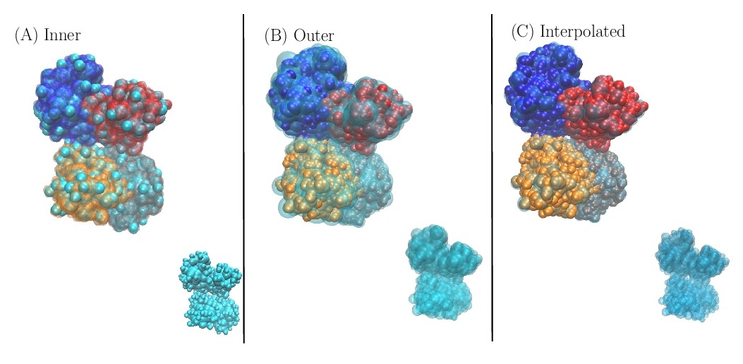
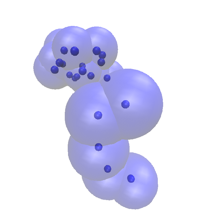
Inner approximation. An approximation by default since the union of the balls defining the approximation is contained within the union of the input particles.
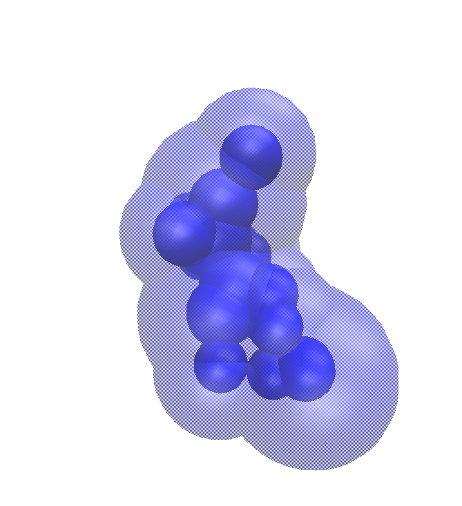
Outer approximation. An approximation by excess since the union of the balls defining the approximation contains the union of the input particles.
Interpolated approximation. An approximation such that its volume matches that of the union of the input particles. The shape defined by the balls is sandwiched between the inner and outer approximations, whence the name interpolated. Such an approximation is termed volume preserving.
As we shall see, volume preserving approximations of atomic models can be obtained using a number of balls equal to 2-5% of the number of atoms.
From Atomic to Coarse Grain Models
Our algorithms are of special interest to coarse grain a molecular geometric model represented by its solvent accessible model.
In this context, we actually provide several alternatives:
(U for Uniform). The coarse-graining is carried out on the volume defined by the solvent accessible model of the molecular geometric model . In doing so, large balls filling the middle of the shape are used – such balls typically cover several amino acids. This strategy is the one of choice if one wishes to compute a geometric approximation of a model, regardless of the size of the balls used.
(A for amino-acids) The coarse-graining is carried out separately on each amino acid of the molecular geometric model . The returned CG model is the union of these local CG models.
One could envision a strategy where one ball would be imposed for each carbon. Doing so would allow defining a covalent structure on the coarse-grain model.
(C for Constrained) A class of models intermediate between and . The coarse-graining is carried out independently on selected a.a., and on their complement. For example, to model cross-linking experiments, one may impose pseudo-atoms to model the exposed LYS separately.
Hierarchical Coarse Grain Models
The aforementioned algorithm can be used iteratively to produce a hierarchy of models. For example, in the context of reconstruction by data integration [5], one may build a hierarchy of coarse-to-fine models. In a first step, one uses the program to compute an interpolated approximation of a molecule with N (=10000) atoms, using n (=1000) balls. Then, one iteratively feeds the balls of the approximation obtained to to obtain an ever simpler approximation of the same volume. For example, starting with N=10,000 atoms and selecting at each step 10% of the balls yields models of size 1000, 100 and 10.
Using Ballcovor: Coarse Graining a Family of 3D Balls
This section describes how to use the program .
Pre-requisites: Volumetric Approximation Schemes
To present the workflow, we specify more carefully the geometric approximation schemes introduced in [47] to approximate a collection of balls by a smaller set of balls (Fig. Geometric approximations).
The following pieces of notation are used in the sequel: if refers to a collection of balls, refers to the corresponding domain i.e. .
Inner approximation Given a 3D model consisting of the union of balls , find a domain , defined by the union of balls , such that the volume of is minimized.
(Concentric) Outer approximation Given a 3D model consisting of the union of balls , find a domain , defined by the union of balls , derived from an inner approximation. The approximation is termed concentric if the balls used to define are concentric with those of an inner approximation.
(Concentric) Interpolated approximation Given a 3D model consisting of the union of balls , find a domain sandwiched between an inner approximation and the associated concentric outer approximation. The approximation is called volume preserving provided that . It is termed concentric if the balls used to define are concentric with those of an inner approximation.
Illustrations on a protein complex consisting of 9060 atoms (PDB id: 1fin)
In this package, we provide a general (and optimal) solution to problem pb-inner-coverering. However, we only address the design of concentric outer and interpolated approximations. The reason for doing so is twofold. First, defining an outer approximation by growing the balls of an inner approximation defines a so-called Toleranced Model (TOM), namely a one-parameter family of shapes obtained by linearly interpolating the radii of the balls between the inner and outer radii. Such models proved instrumental to model large protein assemblies plagued with uncertainties on the shapes and positions of the sub-units [36] , [78] , [79] . Second, as we shall see, growing tight inner approximations produces tight outer approximations.
Input: Specifications and File Types
The main input of is a collection of balls. The file format used is a text file listing the balls. A basic calculation is launched as follows:
The main options of the program are: -fstring: file listing the input family of 3D balls –n-inner-ballsint: number of balls to select in the inner approximation –outer: run the outer approximation –interpolated: run the interpolated approximation
Note that a default radius of is added to all atoms to define the Solvent Accessible Model of the input molecule.
Text file listing the balls in the interpolated approximation
Output files for the run described in section sec-ballcovor-using-balls-input .
Using Ballcovor: Coarse Graining Molecules
This section describes how to use the programs and in different contexts. The pre-requisites being identical to those of , the reader is referred to section Pre-requisites: Volumetric Approximation Schemes .
Input: Specifications and File Types
The main input of is a molecular model loaded from a PDB file. A basic calculation is launched as follows:
The main options of the program are: -fstring: PDB file of the molecule to coarse grain –n-inner-ballsint: number of balls to select in the inner approximation –outer: run the outer approximation –interpolated: run the interpolated approximation
Example Application: Modeling Cross-linking Experiments
We provide one example application of the algorithm . Given a macro-molecular model, cross-link experiments report pairs of LYS which get cross-linked. In order for two LYS to cross-link, two conditions are necessary: these LYS must be exposed, and their distance must be compatible with the size of the cross-linker.
We can therefore use algorithm to design CG models of a molecular model, so as to CG separately the exposed LYS and the atoms of all remaining a.a.
Visualization, Plugins, GUIs
The SBL provides VMD and PyMOL plugins to use the programs of Space_filling_model_coarse_graining . The plugins are accessible in the Extensions menu of VMD or in the Plugin menu of PyMOL . Upon termination of a calculation launched by the plugin, the following visualizations are available:
the inner approximation of the input molecule,
(optionally) the outer approximation of the input molecule,
(optionally) the interpolated approximation of the input molecule.
Algorithms and Methods
In this section, we sketch the algorithms used to compute the three geometric approximations.
Inner Approximation
The main ingredients of the inner approximation are as follows [47] :
the input consists of a collection of balls defining a region ,
from domain , one computes a finite set of balls associated with the medial axis transform of the domain – see package Union_of_balls_medial_axis_3, and defining a covering of , that is, one has . It is important to note that in general, the set is different from the set of input balls .
The algorithm consists of iteratively selecting from the ball providing the best volume increment — a selection done using a priority queue – see package Greedy_selection. Upon selecting a ball say , we recompute the volume increments of the remaining candidate balls intersecting .
Computing the volume of a union of balls is a difficult problem, from a combinatorial, but also numerical standpoint—inverse trigonometric functions are involved. We use our algorithm [46] which returns an interval certified to contain the exact volume – see package Union_of_balls_surface_volume_3.
That is the specification of the algorithm requires a collection of balls defining a region , a selection size or a target ratio between the volume of and that of — that is one expects . The output consists of an ordered set of balls , together with the increment in volume associated to each ball.
Lazy ball selection. One comment is in order about the incremental selection of the ball yielding the best increment, called the dominating ball in the sequel. We perform this operation using the following lazy strategy.
As a pre-processing step, we compute the intersection graph of the candidate balls, namely the graph with one vertex per ball , and one edge for every pair of intersecting balls. Incidences in this graph are used to identify the balls whose volume increment needs to be recomputed.
More precisely:
Step 0. Upon selecting a ball , the remaining candidate balls intersecting are tagged as obsolete.
Step 1. We then pop the top ball from the priority queue and recompute its volume if it is obsolete.
Step 2. If this ball still yields the best increment, it gets selected. Else, the ball is re-inserted into the priority queue, and we move back to step (1).
Outer Approximation
Denote the bounary of the domain . To solve the outer approximation problem, we enlarge the balls from the set , so as to cover the portion of sticking out from .
To see how, recall that the Apollonius diagram of a collection of balls is the Voronoi diagram defined for the following generalized distance [28] :
.
Note that the Apollonius distance is merely the Euclidean distance to the sphere bounding . For each ball of the selection , consider the restriction of the boundary of the input domain not covered yet by the domain , to its Voronoi cell in the Apollonius diagram.
If this restriction is non empty, we define the expansion radius of by the maximum distance of a point of that region to , that is:
If this restriction is empty, the expansion radius is set to the original radius, that is . Expanding each ball of the selection by its expansion radius yields an outer cover of the input domain.
The class T_Space_filling_model_coarse_graining_outer_cover implements this computation without computing the partition of the boundary of the input object induced by the Apollonius Voronoi diagram.
Interpolated Approximation
Consider an inner approximation together with the associated concentric outer approximation, and denote and the inner and outer radii of the i-th ball.
Given a parameter , we define the interpolated radius of the th ball as
An interpolated approximation is the union of these interpolated balls; it is called volume preserving if its volume matches that of the input shape.
Increasing the value of in Eq. eq-interpolated-radius yields nested balls, whence nested interpolated approximations. Therefore, finding the volume preserving interpolated approximation requires a binary search on . Practically, the binary search is stopped when the discrepancy between the volumes is less than .
The class T_Space_filling_model_coarse_graining_interpolated_cover implements this algorithm.
Problem specification: parameters
Input balls defining the domain Selection size Boolean flag to enforce the connectivity of Meshing precision for and
Pre-processing
Compute:
– The Delaunay triangulation of the input balls , and the associated -shape – the vertices of the boundary of – the Delaunay triangulation of these vertices, and the dual Voronoi diagram
– the medial axis of using and , using the algorithm described in [9]
– the balls in defining the covering of , as specified by lemma ???
Is there a refereznce to the covering lemma ?
Inner approximation
– Select the set consisting of balls amidst , using the greedy algorithm from section Inner Approximation
Optional: connectivity enforcement
– Add balls from to enforce the connectivity of , as explained in section ???
Outer approximation
– Mesh the domains and with precision , using the mesher from the CGAL library.
– Compute the expansion radii of the balls in the selection , as specified in section Outer Approximation
Interpolated approximation
– Compute the interpolated radii of the balls defining the interpolated approximation, as specified in section Interpolated Approximation
Computing the inner, outer, and interpolated approximations of a domain defined as a union of balls: overview.
subsection sec-ballcovor-algos-candidate-balls The set of candidate balls
As recalled in section Inner Approximation, the candidate balls defining the set are only centered on the vertices of the medial axis.
subsection sec-ballcovor-algos-volume-selection The volume of the selected balls
More precisely, due to the impossibility to obtain a volume as an exact number type, whatever the kernel used (exact, inexact), the centers and radii of the candidate balls are converted to doubles. These balls are input to our algorithm, which requires two template parameters: the number type of the output (double or interval), and the level of exactness used to compute the constructions involved in the volume computation, namely the coordinates of Voronoi vertices, and boundary points of the union of the selected balls. Following the discussion in [46] , the three options are referred to as (faster, ck_pt_exact and all_exact).
Practically, we use the pair (double, faster) for the inexact kernel, and (interval, all_exact) for the exact kernel.
Programmer's Workflow
The programs of Space_filling_model_coarse_graining described above are based upon generic C++ classes, so that additional versions can easily be developed.
In order to derive such versions, there are two important ingredients, that are the workflow class, and its traits class.


![$t\in [0, 1]$](form_1189_dark.png)


![$t\in[0,1]$](form_1191_dark.png)


