|
Structural Bioinformatics Library
Template C++ / Python API for developping structural bioinformatics applications.
|
|
Structural Bioinformatics Library
Template C++ / Python API for developping structural bioinformatics applications.
|
![]()
Authors: F. Cazals and T. Dreyfus and T. O'Donnell
This package discusses the representations used to represent molecular conformations. Such coordinates are cornerstones of the following tasks [157] , [174] , [97] :
Energy calculations: computing the potential energy of a (macro-)molecular system, using a so-called force field, see the package Molecular_potential_energy.
Structure minimization: minimizing the potential energy of a system by following its negative gradient.
We consider a molecular graph, as introduced in the package Molecular_covalent_structure.
Internal coordinates represent the geometry of a molecule in terms of bond lengths, valence angles, and dihedral angles [141] .
Bond lengths.
Bonds are defined by two points connected in the molecular covalent graph~(Fig. fig-ic-bl-va (A)).
Valence angles.
Valence angles are defined by around a particle participating in two such bonds, thereby defining an angle (Fig. fig-ic-bl-va (B)).
Dihedral angles.
Dihedral angles come into two guises: proper and improper.
For proper angles, consider four consecutive atoms on a path: the dihedral angle in the angle between the two planes defined by the first three and the last three atoms (Fig. fig-ic-dh (A)).
For improper angles, consider a central atom  connected to three atoms, say
  . (Fig. fig-ic-dh (B)). Pick a second atom the define a hinge, e.g.
  to define the hinge
  . The improper dihedral angle is the angle between the planes
  and
and  (Fig. fig-ic-dh (B) ). Note that an improper angle can be thought as the off planarity angle of atom
  with respect to the plane .
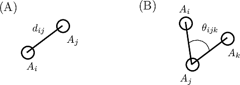 |
| Bond length and valence angle The bond length is the distance between two atoms. The valence angle is the angle at the apex of the triangle formed by two covalent bonds sharing a central atom. |
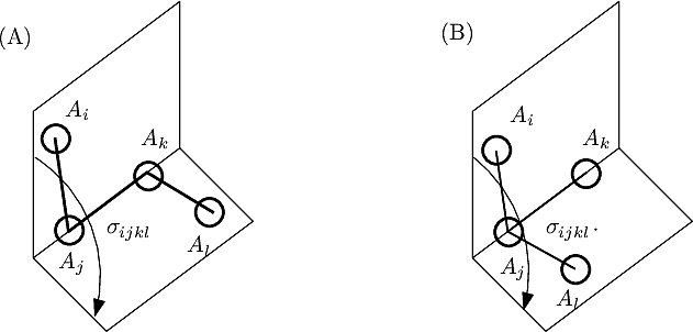 |
| Dihedral angle: proper and improper A proper dihedral angle is defined by three consecutive atoms. An improper dihedral angle is defined by a central atom connected to three others: the angle is that defined by two planes sharing an edge of the tetrahedron involving the four atoms. |
 for example [158] , the semantics of the four tuple
  is as follow:
  is the central atom; the angle is that between the two planes
  and
and  . Note that this amounts to take the pair
  as hinge – even though it may not be a chemical bond.
Internal coordinates are classically represented using a so-called Z-matrix (Z-matrix).
To understand subtleties between the various types of coordinates, the following notations will be useful:
 : number of particles.
 : number of Cartesian coordinates. One has
  .
.
 : number of degrees of freedom. For a non-linear molecules, removing rigid motions (3 degrees of freedom for rotation and translation), one gets
  . (NB: we omit in the sequel the case of linear molecules.)
 : number of primitive internal coordinates. In general, one has
  . This set of coordinates depends on the topology of the molecule studied, see examples exple-ic-cyclobutane and exple-ic-fluoroethylene .
 We now discuss several examples illustrating these definitions.
 , wich results in
  and
and  . However, for case (A), these 6 internal coordinates are three bond lengths, two valence angles, and one dihedral angle. But for case (B), one gets three bond lengths and three valence angles. That is, the internal coordinates available depend on the graph topology.
 . On the other hand,
 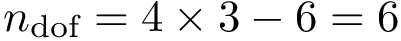 . The following internal coordinates are sufficient to represent uniquely the geometry: four bond lengths, one valence angle, one dihedral angle.
 bond, one can form 4 tuples (whence four dihedral angles) by taking the Cartesian products of the groups of atoms bonded to the two carbons. Thus,
 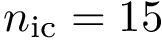 . But since
  , it turns out that the 15 internal coordinates have three redundancies. They can be identified as explained in [15] .
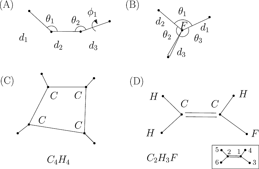 |
| Covalent structure and coordinates: Cartesian coordinates, internal coordinates, and degrees of freedom. See examples exple-ic-one , exple-ic-cyclobutane and exple-ic-fluoroethylene for details. (A) A molecular graph with 4 covalent bond lengths, 2 valence angles, and 1 dihedral angle. (B) A molecular graph with 3 covalent bond lengths and 3 valence angles (C) Cyclobutane: 4 bond lengths, 4 valence angles, 4 dihedral angles. (D) Fluoroethylene: 5 bond lengths, 6 valence angles, 4 dihedral angles. Inset: indices of the atoms for the z-matrix representation of Fig. fig-z-matrix-fluoroethylene . |
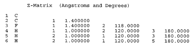 |
| Z-matrix representation of fluoroethylene from Fig. fig-internal-coords-examples (D) (From [15] .) |
C2H3F
APtclcactv11091612353D 0   0.00000     0.00000

  6  5  0  0  0  0  0  0  0  0999 V2000
   -1.0606    0.1723    0.0001 F   0  0  0  0  0  0  0  0  0  0  0  0
    0.1319   -0.4627   -0.0005 C   0  0  0  0  0  0  0  0  0  0  0  0
    1.2458    0.2325    0.0001 C   0  0  0  0  0  0  0  0  0  0  0  0
    0.1690   -1.5420    0.0030 H   0  0  0  0  0  0  0  0  0  0  0  0
    2.1991   -0.2751   -0.0004 H   0  0  0  0  0  0  0  0  0  0  0  0
    1.2087    1.3119    0.0010 H   0  0  0  0  0  0  0  0  0  0  0  0
  1  2  1  0  0  0  0
  2  3  2  0  0  0  0
  2  4  1  0  0  0  0
  3  5  1  0  0  0  0
  3  6  1  0  0  0  0
M  END
$$$$
As illustrated by example exple-ic-fluoroethylene, the choice of a coordinate system to represent a molecule may be non trivial. It is even more so in the presence of cycles. The choice of the representation depends on the problem tackled, and is of paramount importance when geometric optimization (minimization of the potential energy) is carried out. The reader is referred to the excellent overview provided in the Q-Chem user manual (Q-Chem and more specifically here).
In short:
Primitive internal coordinates are encoded in the graph topology. As illustrated by example exple-ic-fluoroethylene, such coordinates are usually redundant, so that deciding of a non redundant set of coordinates does not admit a unique solution. See also [156] .
To reduce the coupling, both harmonic and anharmonic, between internal coordinates, natural internal coordinates were designed [147] , and algorithms to derive them proposed [84] . These algorithms remain complex, though.
internal coordinates, In the sequel, we focus on primitive internal coordinates (PIC) and delocalized internal coordinates (DIC).
Given a molecular graph, see package Molecular_covalent_structure, all primitive internal coordinates are generated as follows:
bond lengths: one iterates over the edges of the graph.
valence angles: one iterates over the pairs of consecutive edges of the graph.
 of the graph; for each edge, one takes the Cartesian products of the particles bonded to a and b, and generate a dihedral angle for each such pair. See for example the four dihedral angles in example exple-ic-fluoroethylene .
 The primitive internal coordinates are computed using the class SBL::CSB::T_Molecular_primitive_internal_coordinates < ConformationType , CovalentStructure >, where ConformationType represents a conformation with Cartesian coordinates as defined in the package Molecular_conformation, and CovalentStructure represents a covalent structure as defined in the package Molecular_covalent_structure.
The class SBL::CSB::T_Molecular_primitive_internal_coordinates provides methods for computing the primitive internal coordinates of :
The class SBL::CSB::T_Molecular_primitive_internal_coordinates provides also methods to fill arrays (or other compliant data structures) with all primitive internal coordinates for :
Equations.
Internal coordinates are defined as follows:
Bond length. The bond length between two particles  and satisfies:

Valence angle. The valence angle at particle is defined by:
Dihedral angle (proper). Denoting  and
and  the normal vectors to the two planes defined by particles
  and particles
  , the dihedral angle is defined by:
Note that the orientations of and determine the sign of the dot product between and , whence the value of  .
.
The two possible orientations of can be illustrated with cis-trans isomerism: in the trans configuration, the dihedral angle is expected to be  , while in the cis configuration, it is expected to be
  .
.
From internal coordinates to Cartesian coordinates.
There exist several strategies to convert back internal coordinates to Cartesian coordinates, and these differ in several respects, namely the number and the type of floating point operations. As shown in [141] , the most efficient one in the so-called SN-NeFR method.
Displacements in internal and Cartesian coordinates are related by the so-called B matrix. To define it, consider:
 :
:  vector of internal coordinates.
 :
:  vector of Cartesian coordinates.
 Following [157] , [97] and the references therein, we define:
 matrix is the
  matrix defined as the Jacobian of the transformation converting Cartesian coordinates into internal coordinates, that is, denoting
  the differential used in multivariate calculus:
Practically, a row of matrix is obtained by differentiating the relevant equation ( Eq. (eq-bond-length) or Eq. (eq-valence-angle) or Eq. (eq-torsion-angle)) with respect to the Cartesian coordinates defining the variable associated with the row.
We cover several embedding operations:
 carbon using distances and valence angles
The operation which consists of computing the Cartesian coordinates of one atom is called the embedding step. This operation requires a context, that is 3 atoms already embedded, with respect to which the new atom is positioned.
This operation is then repeated to embed all atoms.
In the following, we present the  method, from [141].
Given a set of points with  with known embeddings for the first three and the relative position of the fourth (
  ) (Fig. fig-nerf-embedding), the aim is to embed
  .
.
The first operation plainly consists of using spherical coordinates in a suitable coordinate system centered at  }. (Nb: this coordinate system is called specialized reference frame in [7] .) This yields the following coordinates for
  :
:

The second operation consists performing a rotation + translation to transform the previous coordinate system into that of the world/lab. The final position of point reads as

with
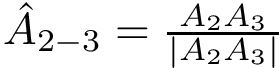 and
and 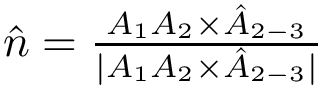
we obtain  :
:
![\begin{equation} R=[\hat{A}_{2-3},\hat{n}\times\hat{A}_{2-3},\hat{n}] \end{equation}](form_716.png)
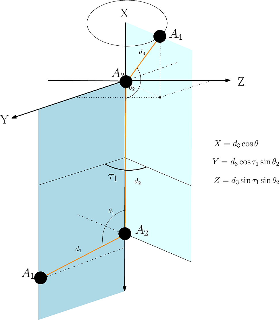 |
| Cartesian embedding of a point given (i) a context defined by three points/atoms, and (ii) a dihedral angle. |
algorithm (Self-Normalizing Natural Extension Reference Frame) [141] simplifies the  method by avoiding normalization operations on vectors. Parallel versions have also recently been proposed, see [7], [18], and [6].
We use the previous operation to iteratively embed a molecule, given all internal coordinates.
Initialization. The initialization consists of embedding three particles connected in a path, using two distances and an angle in an arbitrary Cartesian reference frame. In our case (Fig. fig-from-ic-to-cc):

Iterative embedding of the remaining particles. The embedding of the remaining particles in the coordinate system defined by the first three is computed while performing a traversal of the molecular covalent graph. To describe the algorithm, we use the notion of context, namely three connected atoms which have already been embedded, and with respect to which the new particle is positioned.
The traversal is performed using two stacks: one corresponding to the points to be embedded next; the second one refers to the contexts (one for each atom to be embedded).
Note that the initialization makes it possible to stack all the neighbors of the first three atoms – their context is defined by these three atoms.
Then, the algorithm proceeds iteratively as follows:
The process terminates when the stacks are empty.
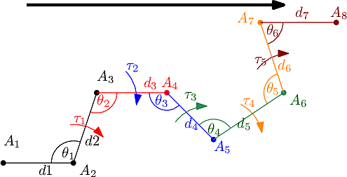 |
| Conversion from internal to Cartesian coordinates. In this illustration the graph is traversed from left to right and each colored particle is embedded using the previous three as context and the three internal coordinates with the same color. |
is that when computing  , no normalization is used as it equals 1 by construction. Whence the Self-Normalizing Natural Extension Reference Frame name. Also the norm
  used when embedding a point is stored as the points of the covalent graph are embedded such that it is not recomputed.
Implementation: main class. The conversion is performed using the operator of class SBL::CSB::T_Molecular_cartesian_coordinates. The template arguments are the Conformation type and the Covalent structure. As parameter for the operator the covalent structure and the internal coordinates are required (bond lengths, bond angles and dihedral angles).
Implementation: utilities. Static functions are defined in SBL::CSB::Molecular_coordinates_utilities. These can be used to compute bond and dihedral angles given vectors and to embed a particle given three others and internal coordinates as done in .
To graft the carbon of a side chain on a known backbone, one uses the following internal coordinates:
 . The half-angle is denoted
  .
. . We also denote
  .
.Analytically, define the following –see [odonnell2022modeling] :

One obtains the two possible embeddings for :
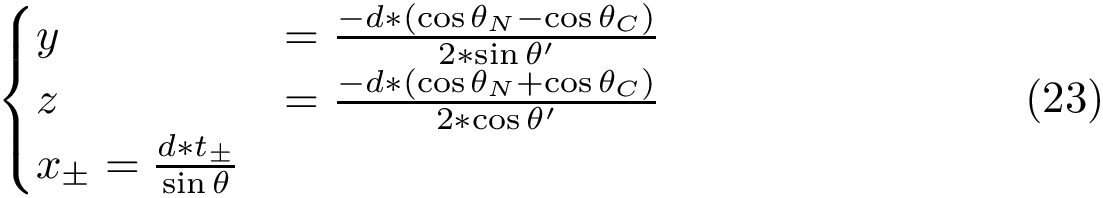
is to use an improper dihedral angle with respect to the plane  . However, because in force fields the force constants are much stiffer for valence angles (and bond lengths), the solution which respects two valences angles is preferable.
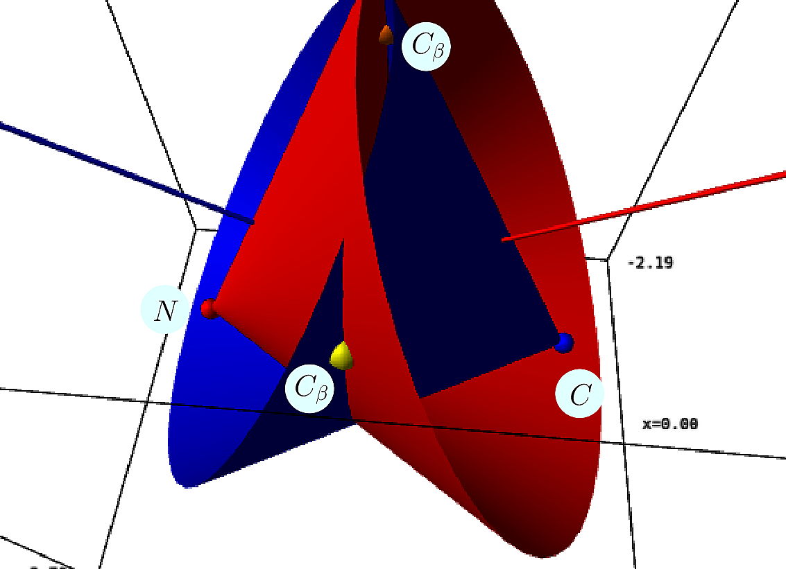 | 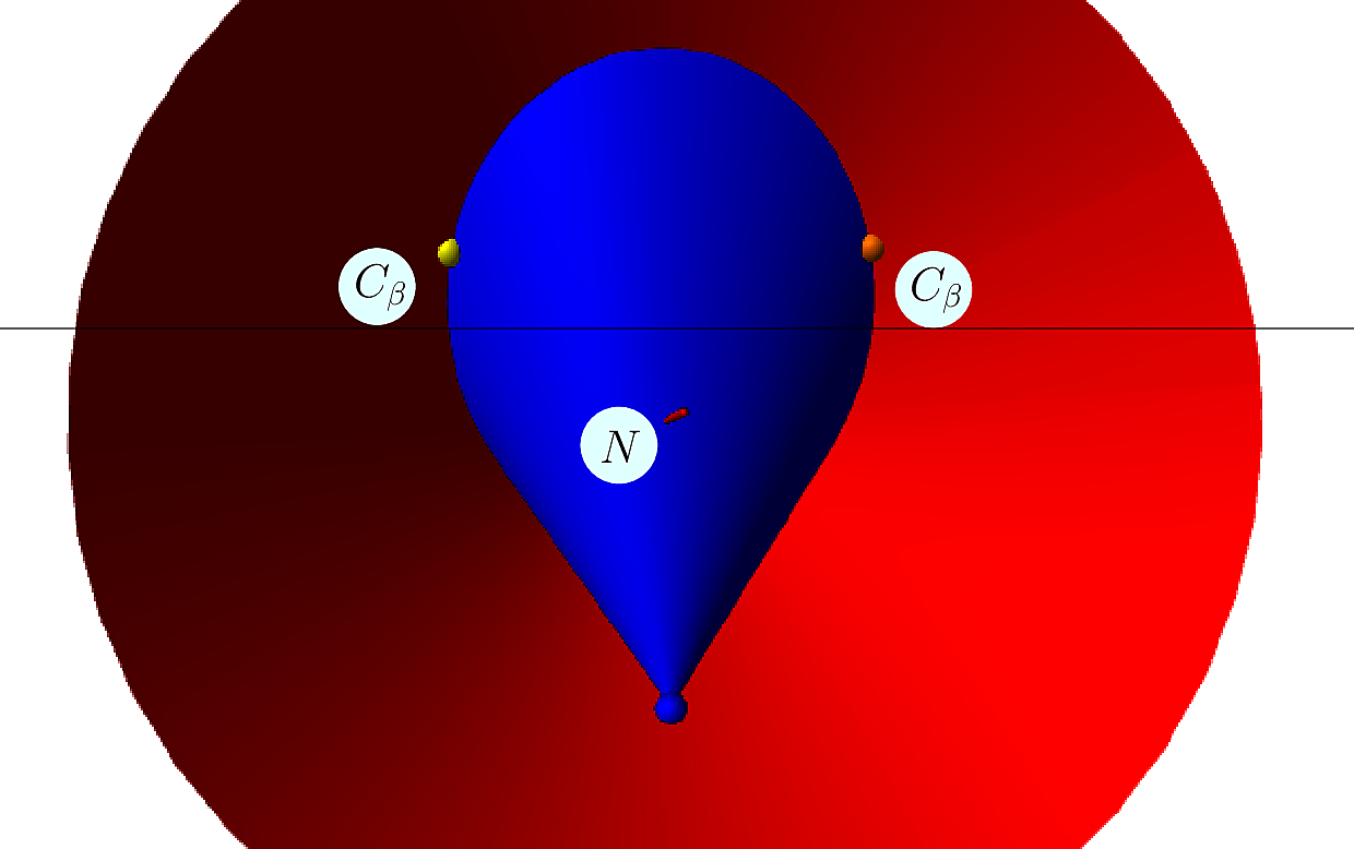 |
| Placing the carbon. Using three valence angles and one distance yields two solutions, the correct one being selected by a chirality argument. |
The correct solutions is selected by chirality, noting that the volume of the tetrahedron defined by  is positive – in known structures.
To derive the DIC, we follow [15] :
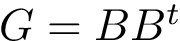
2. Extract the eigenvector/values of  . Denote
  the num. of
  eigenvalues. Typically,
  .
.
Denote  and , respectively, the eigenvectors associated to strictly positive and null eigenvalues. The eigen equation of satisfies
![$G (U R)= (U R) \left[ \begin{array}{c|c} \Lambda & 0 \\ \hline 0 & 0 \end{array} \right]$](form_735.png)
One may say that:
: spans the non redundant subspace of the original space of primitive coordinates : spans the redundant subspace.
And their derivatives.
For the gradient in internal coordinates, see [157] , [97] and the references therein.
This package offers also offers sbl-coordinates-converter.exe and sbl-coordinates-file-converter.exe to perform various conversions of coordinates.
The application sbl-coordinates-converter.exe provides the following conversions:
We note in passing that our encoding of internal coordinates is based on atom ids, as provided in PDB files.
Converting Cartesian coordinates to internal coordinates. Given a PDB file, this executable generates all IC (bond lengths, valence angles, dihedral angles):
sbl-cartesian-internal-converter.exe --pdb-file data/ala5.pdb
This call simply generates one txt file for each type of coordinate:
==> ala5_bonds.txt <==
#Chain X
#Atom ids bond length(Angstrom)
1 5 1.45994
5 11 1.51006

==> ala5_bond_angles.txt <==
#Chain X
#Atom ids bond angle(radii)
5 1 2 1.90268
5 1 3 1.90217

==> ala5_dihedral_angles.txt <==
#Chain X
#Atom ids dihedral angle(radii)
2 1 5 11 0
2 1 5 7 0.979966
Converting internal coordinates into Cartesian coordinates: all coordinates provided. A simple case is that were all IC are provided. In that case, one needs to provide
sbl-cartesian-internal-converter.exe --pdb-file ala5.pdb --bond-lengths-file ala5_bonds.txt --bond-angles-file ala5_bond_angles.txt --dihedral-angles-file ala5_dihedral_angles.txt
This call simply generates a txt file containing the Cartesian coordinates – ala5_cartesian.txt in the previous example.
Converting internal coordinates into Cartesian coordinates: selected coordinates missing. In case selected IC are missing, a force field can be passed so as to use the equilibrium values of the corresponding models. For example, using  :
:
sbl-cartesian-internal-converter.exe --pdb-file ala5.pdb --bond-angles-file ala5_bond_angles.txt --dihedral-angles-file ala5_dihedral_angles.txt --force-field-file data/amber-ff14sb.xml
The executable sbl-coordinates-file-converter.exe convertes xtc files to the Point_d format. This conversion is useful by several executables from the SBL – see e.g. the package Landscape_explorer .