|
Structural Bioinformatics Library
Template C++ / Python API for developping structural bioinformatics applications.
|
|
Structural Bioinformatics Library
Template C++ / Python API for developping structural bioinformatics applications.
|
Authors: F. Cazals and T. Dreyfus and C. Roth
![]()
This package provides methods to assess the conformational diversity of an ensemble of conformations.
Consider a sampling – aka conformational ensemble, as defined in section Conformational ensembles – aka samplings. This package offers functionalities to:
Assessing the structural diversity of the sampling, using various statistics:
Perform a hierarchical clustering of the conformations.
These functionalities are provided in the program  .
.
Currently we use two measures for the sampling diversity, in order to assess the extent to which a molecule deforms within an ensemble  . Assume that all conformations have been aligned in the same coordinate system, see Eq. eq-aligned-conformations.
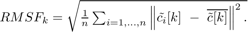
The first is the standard method for estimating the root-mean squared atom fluctuations (  ). Denoting
  the average position of the
  -th atom in the aligned samples
  . The of the -th atom is defined by
The second measure is the bounding box (in Cartesian coordinates) of the ensemble of aligned structures.
A conformational ensemble may contain clusters , i.e. groups of conformations such that pairwise distances within a cluster are smaller than distances between conformations across clusters. We investigate such properties using graphs.
Assume that a connected nearest neighbor graph (NNG, see Def. def-nng)  has been built over the samples, and denote
  (resp.
  ) its vertex set (resp. its edge set). Assume that to each edge
 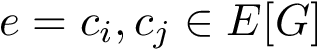 is attached the quantity
 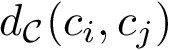 . We compute a minimum spanning tree
  of . If the conformational ensemble contains
  conformations, this tree involves
  edges. For an edge
  of this graph, the edge length is the distance between the conformations
  and
and  , that is . Denoting
  the edge set of the MST, and
  a particular edge, we then report the following statistical summary for :

To intuitively capture the significance of this summary, consider the situation where the ensemble has a cluster structure, with dense regions separated by mostly empty space. In that case, most of the edges are short ones, only those connecting clusters being long ones, which reads plainly from the statistical summary.
When an ensemble features clusters, as e.g. seen from the statistical summary from the edge lengths found in a MST, the next step consists of finding these clusters. Upon estimating the sample density at each sample from the ensemble, a three stage strategy consists of associating one cluster to each local maximum of the estimated density [53] , [93], and to filter out spurious (i.e. small) ones. We now briefly review these steps.
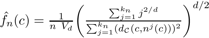
The first task is the density estimation. Assume that a nearest neighbors graph (NNG) has been built, so that each sample is linked to a number of its nearest neighbors, say its nearest neighbors. Intuitively, the density about a sample is inversely proportional to the distances to the nearest neighbors. Formally, denoting the number of nearest neighbors and  the volume of the unit ball in
  , the local density at sample can be estimated as [22] :
To define clusters, consider the lifted NNG obtained by endowing each sample with the previous estimated density. We define a cluster as the catchment basin (watershed) associated with a local maximum of the estimated density [52] . Along the way, spurious local maxima are filtered out using topological persistence [52] .
Prosaically, this process is analogous to that used in topography to define a peak on a mountain range: a peak  is persistent if the elevation drop to the saddle leading to a higher peak, say
  , is at least some user defined value. If not, the peak may be considered as a secondary peak of . The user is referred to the package Morse_theory_based_analyzer for further details.
Computing pairwise distances between (selected) conformations, so as e.g. to run a dimensionality reduction algorithm such as multi-dimensional scaling or Isomap. Such low dimensional embeddings are indeed highly convenient to visualize the relative position of a set of conformations, e.g. low lying local minima.
To this end, we proceed in two steps:
First, all conformations are aligned in the same coordinate system, as specified by Eq. eq-aligned-conformations.
The input is a list of conformations of the same molecule, and can be provided with several format:
6 x11 y11 z11 x12 y12 z12
6 x21 y21 z21 x22 y22 z22
6 x31 y31 z31 x32 y32 z32
...
It is also possible to provide an XML archive containing a boost graph representing the precomputed nearest neighbours graph (in order to skip the sometimes time consuming construction of the nng). All analysis are optional, so that they have to be specified in the command-line. For example, running analysis over the sampling diversity is done using the option –sampling-diversity. Note that all other analysis require the computation of the nng, meaning that the option –nng-builder should be used. Thus, a calculation is launched as follows:
> sbl-conf-ensemble-analysis-lrmsd.exe --points-file data/bln69_sampling.txt --sampling-diversity --pairwise-distances --nng-builder --num-neighbors 10 --mst --mtb --directory results --verbose --output-prefix --log
are:–points-file string: plain text file listing all conformations as D-dimensional points–sampling-diversity: run Sampling Diversity Analysis–nng-builder: run the NNG Builder–num-neighbors int: Target number of neighbors for each vertex–mst: run Minimal Spanning Tree Analysis–mtb: run Morse Theory Based Analysis
| File Name | Description |
| BLN69 conformations file | Sampling done from sbl-landexp-hybrid-BH-TRRT-BLN.exe |
| Preview | File Name | Description |
General: log file, sampling diversity and sampling sparsity | ||
| Log file | Log file containing high level information on the run of | |
| Analysis xml file | Global analysis serialized using Boost into an XML archive | |
Module pairwise distances | ||
| Distances plain text file | Matrix of pairwise distances | |
Module NNG builder | ||
| NNG xml file | NNG serialized using Boost into an XML archive | |
Module MTB analysis: persistence based clustering | ||
| Morse Smale Witten chain complex xml file | Morse Smale Witten chain complex serialized using Boost into an XML archive | |
| Stable manifold partition xml file | XML archive listing the samples repartition by persistent basin | |
| Disconnectivity forest image file | Disconnectivity forest drawn in eps file format | |
| Sorted basins plain text file | List of all basins sorted by persistence | |
| Persistence diagram plot script | Gnuplot script for the persistence diagram | |
| Persistence diagram image | Persistence diagram drawn by gnuplot in pdf file format | |
| Persistences plain text file | List of all finite persistences | |
| Persistence histogram plot script | R script for the persistence histogram | |
| Persistence histogram image | Persistence histogram drawn by R in pdf file format | |
Computing these measures requires performing a registration of each conformation into a unique coordinate system, as specified in Eq. (eq-aligned-conformations).
Using the first conformation  as reference, one can transform every other conformation by applying to it the rigid transform defining the
  between and .
Extracting the MST out of a connected graph is a classical problem in computer science. We use Prim's algorithm, which iteratively attaches one node not connected yet, namely that using the shortest edge available which does not create a cycle.
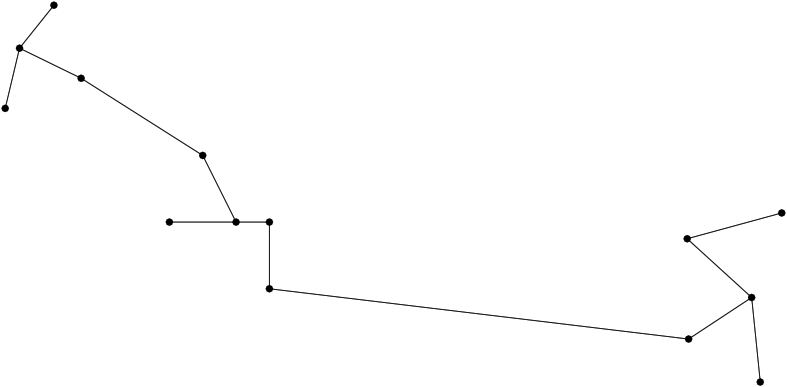 |
| A minimum spanning tree (MST) connecting conformations The MST is computed once all conformations have been registered in the same coordinate system. The distribution of edge lengths provides information on the sampling density. |
Once the density has been estimated (Eq. eq-estimated-density), the persistence based clustering is carried out using the algorithms implemented in the package Morse_theory_based_analyzer. See also the module MTBA in the workflow of section Algorithms and Methods.
Changing the representation used for conformations.
In order to derive such versions, there are two important ingredients, that are the workflow class, and its traits class, as we shall see now.
T_Conformational_ensemble_analysis_traits:
T_Conformational_ensemble_analysis_workflow: